1. Introduction
Solubility in water is among the first properties a medicinal chemist asks about a new compound. A poorly soluble molecule is difficult to dose orally, gives unreliable readings in biochemical assays, and complicates every later stage of development. Because measurement consumes material and time, the appeal of calculating the value from structure has been constant. Jorgensen and Duffy (2002) surveyed the computational approaches available at the turn of the century and set out the practical reasons for wanting them, and the problem has stayed on the agenda of cheminformatics ever since.
The modelling strategy has shifted substantially. Early schemes computed solubility from a small number of interpretable descriptors, most famously the general solubility equation, which relates the logarithm of molar solubility to the octanol-water partition coefficient and the melting point (Yalkowsky and Valvani, 1980; Ran and Yalkowsky, 2001). Later work replaced hand-chosen descriptors with fixed-length fingerprints and a regression model. The current generation dispenses with the fingerprint and learns a representation from the molecular graph itself, using the message passing machinery introduced for quantum chemical property prediction by Gilmer et al. (2017).
This article reviews what the published literature supports about that third generation. It is a narrative review of the methodological and benchmarking work rather than an exhaustive survey, and it makes no claim to a systematic search. The questions it addresses are three. What do graph neural networks actually do differently on this task? What do the benchmarks and the blind challenges show about their accuracy relative to simpler methods? And which parts of the remaining error are attributable to the models as opposed to the data they are trained and judged on?
2. How the Problem Is Posed
Almost all published models predict the base-ten logarithm of solubility in moles per litre, written logS. Two quantities travel under that name and they are not interchangeable. Intrinsic solubility refers to the neutral form of the compound in equilibrium with its most stable solid phase. Apparent or kinetic solubility refers to what is measured when a concentrated stock in an organic solvent is diluted into buffer, a procedure that is faster, more relevant to assay conditions and often yields a higher number because the precipitate has not had time to order itself. Models fitted to one target and evaluated against the other will appear worse than they are.
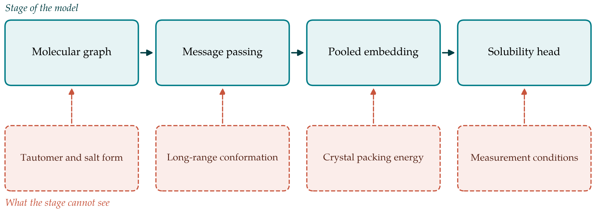
The structural input is almost always a connection table expressed as SMILES (Weininger, 1988). That input carries the atoms, the bonds and the formal charges. It does not carry the solid form, which is the property on the other side of the thermodynamic cycle that determines intrinsic solubility, and it does not uniquely determine the tautomer or the protonation state at a given pH. Any model reading structure alone is therefore solving an underdetermined problem, and the extent of that underdetermination sets a floor on achievable accuracy that no amount of training data removes.
Training sets have historically come from compilations of literature values. The dataset accompanying the ESOL model of Delaney (2004) remains in wide use, as does the solubility task within MoleculeNet (Wu et al., 2018), which packages several property prediction sets with suggested splits. Both aggregate measurements made in different laboratories by different methods, and Palmer and Mitchell (2014) argued that the resulting label noise, rather than the modelling, accounts for much of the error that published studies report.
3. From Descriptors to Learned Graph Representations
Three families of model appear in the literature, and they differ less in their mathematics than in where the representation comes from. Table 1 sets them beside one another with the kind of evidence each rests on. The first family computes physically motivated descriptors and fits a small regression. The second computes a fixed topological fingerprint, typically extended connectivity fingerprints (Rogers and Hahn, 2010), and fits a random forest or gradient boosting model to it. The third learns the representation.
| Family | Representation | Typical strength | Typical weakness |
|---|---|---|---|
| General solubility equation | logP and melting point | Interpretable; grounded in thermodynamics (Yalkowsky and Valvani, 1980) | Needs a measured melting point |
| Group contribution | Counted fragments and corrections | Transparent; fast (Delaney, 2004) | Blind to context beyond the fragment |
| Fingerprint regression | Fixed circular fingerprint | Strong baseline; cheap to retrain (Rogers and Hahn, 2010) | Bits are not tuned to the endpoint |
| Graph convolution | Learned atom and bond features | Differentiable fingerprint (Duvenaud et al., 2015) | Needs more data to fit |
| Message passing network | Learned bond-directed messages | Best reported accuracy on several tasks (Yang et al., 2019) | Sensitive to split and to label noise |
| Attention-based graph model | Weighted neighbourhood aggregation | Weights can be inspected (Xiong et al., 2020) | Interpretation is suggestive, not causal |
The learned family began with the differentiable fingerprint of Duvenaud et al. (2015), which reproduced the circular fingerprint algorithm with continuous, trainable operations so that the representation could be optimised for the endpoint. Gilmer et al. (2017) then showed that most such architectures, along with graph convolutional networks of the kind described by Kipf and Welling (2017), are instances of a single message passing scheme: atoms exchange messages with bonded neighbours for a fixed number of rounds, and a readout function pools the resulting atom vectors into one molecular vector. The directed bond variant implemented in the work of Yang et al. (2019) is the version most often used for solubility, and attention weighting of the neighbourhood, as in the model of Xiong et al. (2020), is a common refinement.
Two consequences follow from the message passing structure. The receptive field of an atom after k rounds is the set of atoms within k bonds, so three or four rounds capture substituent effects but not the relationship between two ends of a long molecule. And because the molecular vector is a sum or mean over atoms, properties that depend on the arrangement of the whole molecule in space, including the way it packs into a crystal, have no natural route into the representation. Figure 1 places these limits against the stages of the model.
4. What the Benchmarks Show
Benchmark results on curated sets favour the learned models, but by margins that are smaller than the architectural literature sometimes implies. The MoleculeNet comparison of Wu et al. (2018) reported graph-based methods ahead of fingerprint baselines on the solubility task, and the systematic comparison by Yang et al. (2019) found a directed message passing network ahead of descriptor and fingerprint models across a range of datasets, while also noting that concatenating computed global descriptors onto the learned vector improved results further. That last observation is worth keeping in view: the learned representation did not make the physical descriptors redundant.
Blind challenges give a harder test because the answers are withheld. The first solubility challenge (Llinas et al., 2008) asked participants to predict intrinsic solubilities for a small set of druglike molecules from a consistent set of measurements, and the second challenge (Llinas et al., 2020) repeated the exercise with two test sets of differing measurement quality. The reported outcome of both exercises was sobering relative to the errors quoted in retrospective studies, and performance tracked the reliability of the reference measurements as much as the sophistication of the method.
Split design accounts for part of the gap between retrospective and prospective accuracy. Random splits place close analogues on both sides of the partition, so a model that has memorised a series can appear to generalise. Sheridan (2013) made the case for time-based splits as a closer analogue of prospective use, and scaffold splits serve a similar purpose in the benchmark suites assembled by Wu et al. (2018) and by Hu et al. (2020). Reported errors under scaffold splitting are consistently larger, and comparisons that mix split types are not informative.
5. Where the Remaining Error Comes From
Three sources of error are distinguishable in the literature and they call for different responses. The first is label noise. Aggregated literature solubilities differ between laboratories for reasons that include the solid form used, the equilibration time, the buffer and the analytical method, and Palmer and Mitchell (2014) treated the resulting spread as a bound on what any model fitted to such data can achieve. A model cannot be more consistent than its labels, and reporting an error substantially below the reproducibility of the measurement should prompt a check of the split rather than satisfaction.
The second is the missing solid state. Intrinsic solubility depends on the free energy of the crystal as well as on solvation, which is why the general solubility equation needs a melting point (Ran and Yalkowsky, 2001). Topological models are given no information about polymorph, lattice energy or salt form, so a pair of compounds differing only in crystal behaviour is, to the model, nearly the same molecule. This is a representational limit and not a training deficiency.
The third is chemical domain. Models extrapolate poorly to scaffolds, charge states and size ranges absent from training, and the practical consequence is that a model useful on a company series may be of little use on an unrelated chemotype. The wider discussion of expectations in machine learning for drug discovery, including the observations of Walters and Murcko (2020), applies squarely here: the question for a prospective user is not which architecture scored best in a paper but whether the compounds of interest resemble the training set. Mitchell (2014) made the same point about applicability domain for cheminformatics models generally.
6. Gaps and Directions
The clearest gap is measurement. Curated sets produced under one protocol, with the solid form characterised and the pH recorded, are worth more than larger aggregated compilations, and the two solubility challenges showed how much turns on that distinction (Llinas et al., 2020). Publishing failed and borderline measurements alongside successful ones would help further, since models trained only on compounds soluble enough to measure easily inherit that selection.
A second direction is calibrated uncertainty. A prediction accompanied by an honest interval is usable in triage even when the central estimate is imperfect, and ensembles or conformal methods give this at modest cost. A third is the hybrid route already visible in the results of Yang et al. (2019), in which physically meaningful descriptors are supplied alongside the learned graph vector, so that knowledge which the graph cannot encode enters by another door. Work that couples predicted or measured melting behaviour to a graph model follows the same logic.
Finally, evaluation practice could be tightened at little cost. Reporting the split type, the composition of the test set, the measurement protocol behind the labels and the performance of a fingerprint baseline would make the literature far easier to read. Shared infrastructure of the sort assembled by Hu et al. (2020) has improved comparability in adjacent areas, and the same discipline applied to solubility would clarify how much of the reported progress is real.
7. Conclusion
Graph neural networks have changed how aqueous solubility is modelled, replacing fixed fingerprints with representations tuned to the endpoint, and on curated benchmarks they generally edge out the older methods. The published record does not, however, support the view that the problem is now solved by architecture. Blind challenges and scaffold-based splits place accuracy well short of retrospective figures, careful descriptor and fingerprint baselines remain close, and the two factors that limit performance most, namely the heterogeneity of literature solubility data and the absence of the solid state from a topological description, are untouched by deeper networks. Progress is more likely to come from better measurements, honest splits and calibrated uncertainty than from further variation on the message passing theme.
Conflict of interest
To be declared by the author(s) before publication.
Funding
To be declared by the author(s) before publication.