1. Introduction
The Laplacian matrix of a weighted graph is the difference between the diagonal matrix of weighted degrees and the matrix of weights. Its spectrum encodes a great deal of structure. The multiplicity of the eigenvalue zero counts connected components, the second smallest eigenvalue, which Fiedler (1973) named the algebraic connectivity, measures how well the graph hangs together, and the corresponding eigenvector suggests where to cut it (Mohar, 1991; Merris, 1994; Chung, 1997). These facts are the basis of spectral clustering (von Luxburg, 2007) and of the analysis of synchronisation by master stability functions (Pecora and Carroll, 1998).
Multilayer networks extend the single graph to a family of graphs, the layers, whose nodes are linked across layers as well as within them. The general formalism is set out by De Domenico et al. (2013) and Kivelä et al. (2014), and the review of Boccaletti et al. (2014) covers structure and dynamics. For the Laplacian, the key findings are those of Gómez et al. (2013), who showed that diffusion on a multiplex can be faster than on any of its layers, of Solé-Ribalta et al. (2013), who described the spectrum in the limits of weak and strong coupling, and of Radicchi and Arenas (2013), who found that the passage between the two limits is abrupt.
Those results concern idealised settings, typically two layers with a single coupling constant. An analyst facing a weighted network with several layers and unequal couplings has to decide how to build the matrix, what to compute, and how to tell a property of the system from an artefact of those decisions. This article proposes a framework for doing so in a consistent and reportable way. The framework is assembled from the published theory. It is not applied to a data set here, and no numerical findings are reported.
2. Setting and Notation
Consider M layers on a common set of N nodes. Layer α has a symmetric matrix of nonnegative intralayer weights and a Laplacian L(α). The copy of node i in layer α is joined to its copy in layer β by an interlayer
αβ, which may be zero. The supra-Laplacian L is the Laplacian of the weighted graph on link of weight ci the NM node-layer pairs. It is the sum of two positive semidefinite matrices: an intralayer part, block
αβ. When the diagonal with the layer Laplacians as blocks, and an interlayer part built from the weights ci interlayer weights do not depend on the node and equal p times the weights of a graph on the layers with Laplacian LI, the interlayer part is the Kronecker product of pLI with the identity of order N (Solé-Ribalta et al., 2013). Eigenvalues are written in increasing order, starting from λ1 = 0.
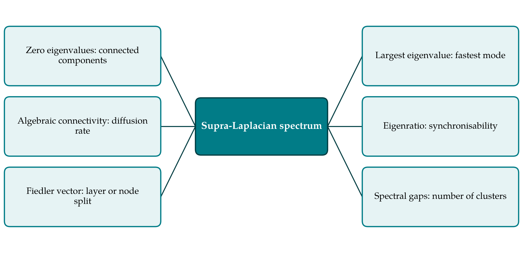
Figure 1 gathers the spectral quantities that the framework is meant to deliver and the interpretation usually attached to each. For the diffusion equation x′ = −Lx the slowest decay rate is λ2 (Gómez et al., 2013); for identical oscillators coupled through L, the ratio of the largest eigenvalue to λ2 determines how wide the range of coupling strengths compatible with synchrony can be when the master stability function is negative on a bounded interval (Pecora and Carroll, 1998).
3. The Proposed Framework
The framework consists of seven stages, listed in Table 1 with the product of each. The stages are meant to be carried out in order, and the bounds of the fourth stage serve as checks on the computations of the fifth.
| Stage | What is done | Product |
|---|---|---|
| 1. Specification | State layers, node alignment, weights and their units | Written model description |
| 2. Assembly | Build intralayer and interlayer parts as separate sparse matrices | Supra-Laplacian with a coupling parameter |
| 3. Structural checks | Test symmetry, sign of weights, zero row sums, connectedness | Number of components per layer and overall |
| 4. Bounds | Apply Gershgorin, Weyl, test-vector and interlacing bounds | Intervals for the eigenvalues of interest |
| 5. Computation | Compute the required eigenpairs with a method suited to the size | Eigenpairs with residual norms |
| 6. Coupling sweep | Follow eigenvalues and eigenvectors as the coupling varies | Regimes and crossover coupling |
| 7. Comparison and sensitivity | Compare with layers, aggregate and reweighted networks | Statement of what is specific to the system |
3.1. Specification and assembly
The first stage fixes what the matrix means. Intralayer and interlayer weights often have different origins, for example flows along routes and transfer rates between modes, and are then not measured in the same units. Their ratio is a modelling choice, and the framework treats it as an explicit parameter p multiplying the interlayer part, to be varied in the sixth stage and never fixed silently. The specification also states whether every node is present in every layer, and whether the combinatorial Laplacian or a degree-normalised form is intended; the normalised form corresponds to random walks and has its spectrum in a fixed interval (Chung, 1997). Assembly keeps the two parts as separate sparse matrices so that L can be formed for any p without rebuilding.
3.2. Structural checks and bounds before computation
The third stage verifies the properties on which everything else rests: symmetry, nonnegative weights and zero row sums. It then counts connected components of each layer and of the whole multilayer graph by graph search. The number of components equals the multiplicity of the eigenvalue zero, and knowing it in advance tells the analyst how many trivial eigenpairs to deflate and which eigenvalue is the first informative one.
The fourth stage produces bounds that cost almost nothing. Gershgorin's theorem bounds the largest eigenvalue by twice the largest weighted degree of a node-layer pair. Weyl's inequalities, applied to the splitting into intralayer and interlayer parts, place the k-th eigenvalue of L between the k-th eigenvalue of the intralayer part and that value plus the largest eigenvalue of the interlayer part (Horn and Johnson, 2013). Rayleigh quotients of well-chosen test vectors give upper bounds on λ2. With node-independent coupling, vectors constant within each layer are eigenvectors, so the numbers p times the eigenvalues of LI belong to the spectrum; for two layers this is the eigenvalue 2p. Vectors that repeat the same node pattern in every layer show that λ2 is at most the algebraic connectivity of the average of the layer Laplacians. Finally, the eigenvalues of suitably normalised quotient graphs, the aggregate network over nodes and the network of layers, interlace those of L (Sánchez-García et al., 2014).
3.3. Computing the relevant eigenpairs
Only a small part of the spectrum is normally needed: the few smallest nonzero eigenvalues with their eigenvectors, and the largest eigenvalue. For matrices of order up to a few thousand a dense symmetric eigensolver returns everything reliably (Golub and Van Loan, 2013). Beyond that, sparse iterative methods are required. The implicitly restarted Lanczos method in ARPACK (Lehoucq et al., 1998) finds the largest eigenvalue directly and the smallest ones in shift-and-invert mode; since L is singular, a small negative shift makes the shifted matrix positive definite and allows a sparse Cholesky factorisation. The block method of Knyazev (2001) avoids factorisation, accepts a preconditioner, and can be constrained to the complement of the known null vectors.
Each computed pair is accepted only with its residual norm, which for a symmetric matrix bounds the distance from the computed value to a true eigenvalue. Eigenvectors are less robust: their sensitivity grows as the gap to neighbouring eigenvalues shrinks (Stewart and Sun, 1990), and near a crossing of eigenvalues an individual vector is not meaningful, only the invariant subspace is. The computed values are then confronted with the intervals from the fourth stage, and a violation indicates an error in assembly or an unconverged computation.
3.4. Sweeping the interlayer coupling
The sixth stage repeats the computation over a logarithmic grid of values of p spanning the range from coupling much weaker than the intralayer weights to much stronger. Theory predicts the two ends. For weak coupling, and connected layers, the smallest nonzero eigenvalues grow linearly in p and their eigenvectors are nearly constant within layers, so the layers act as units. For strong coupling the copies of each node lock together and the low end of the spectrum approaches that of the averaged Laplacian (Gómez et al., 2013; Solé-Ribalta et al., 2013). In the two-layer case with a single coupling constant, Radicchi and Arenas (2013) showed that λ2 equals 2p exactly up to a critical coupling, beyond which it follows a different branch, and that the critical value is at most one quarter of the algebraic connectivity of the sum of the two layer Laplacians.
To locate the regimes in a weighted network with several layers, the framework recommends tracking two numbers along the sweep: the gap between λ2 and its linear weak-coupling prediction, and the share of the squared norm of the Fiedler vector carried by its layer-wise averages. The second quantity is close to one when the vector separates layers and close to zero when it separates groups of nodes. Branches are followed through near-crossings by matching eigenvectors between consecutive values of p by their overlap. With unequal interlayer weights there may be no exact crossing, and the change is then reported as a range of p.
3.5. Reference comparisons and sensitivity
A spectral quantity is informative about the multilayer structure only in comparison. The seventh stage computes the same quantities for each layer alone, for the aggregate network obtained by summing the layers, and for versions of the network in which intralayer weights are permuted among existing links, which preserves topology and destroys the correlation between weight and position. Sensitivity to individual weights follows from first-order perturbation theory: for a simple eigenvalue with unit eigenvector v, the derivative with respect to the weight of the link between a and b is the square of va − vb (Stewart and Sun, 1990). The derivative is never negative, in agreement with the monotonicity of Laplacian eigenvalues under added weight, and ranking links by it identifies those whose measurement error matters most.
4. Fitting the Framework to an Application
What is reported depends on the question. For diffusion or consensus the quantity of interest is λ2 as a function of p, set against the layers and the aggregate. For synchronisation it is the eigenratio. For partitioning it is the Fiedler vector and the next few eigenvectors, with the caution about small gaps noted above. In every case the report should give the specification of the first stage, the component counts, the bounds, the solver and its residuals, and the grid of couplings, so that the analysis can be repeated. Networks in which nodes are absent from some layers need one adjustment: test vectors that repeat a node pattern across layers are no longer available, and the aggregate bound is replaced by the interlacing statement for the quotient.
5. Limitations and What Remains to Be Shown
The framework is proposed and has not been validated here. It organises results that are proved in the cited literature, but its usefulness depends on matters that only applications can settle: whether the regime indicators of the sixth stage remain clear when interlayer weights are strongly heterogeneous, how fine the grid of couplings must be, and whether the reference networks of the seventh stage are the right ones for a given field. A study applying the framework to several weighted multilayer data sets of different origin would be needed to answer these questions.
There are also limits of scope. Everything here assumes symmetric weights. Directed layers lead to nonsymmetric Laplacians with complex eigenvalues, for which the variational bounds and the residual test do not hold in the same form. Time-varying layers, signed weights and interlayer links between different nodes fall outside the setting as well, although the stages of specification, structural checking and comparison carry over.
6. Conclusion
The spectrum of the supra-Laplacian is a compact summary of how a weighted multilayer network diffuses, synchronises and divides, but only if it is clear how the matrix was built and what the numbers are measured against. The framework proposed in this article separates the analysis into stages, places inexpensive bounds before computation, treats the interlayer coupling as a parameter to be swept, and ends with reference comparisons and a sensitivity analysis. It relies on established theorems throughout, and its practical value is a matter for applied work to determine.
Conflict of interest
To be declared by the author(s) before publication.
Funding
To be declared by the author(s) before publication.