International Journal of Signal Processing

Sparse Recovery of Wideband Spectra From Sub-Nyquist Samples Under Impulsive Noise: A Review of Methods

Keisha Oliveira¹, Jelena Grant², Vikram Afolabi³

¹ Department of Electrical Electronics, Rhine University Centre for Electrical Electronics, New Zealand, ² Department of Electrical Electronics, Transylvanian Center for Electrical Electronics, Kazakhstan, ³ Department of Electrical Electronics, Tagus University Centre for Electrical Electronics, Spain

Published 31 Jul 2026 Vol. 1, Article 1 10.62715/ijsp.2026.v1.i1.pp1-7 0 accesses 0 citations

Download PDF XML HTML EPUB

0Accesses

0Citations

Abstract

Wideband spectrum sensing asks a receiver to locate the occupied bands in a frequency range too wide to digitise at the Nyquist rate. Compressed sensing made this possible in principle: when only a few bands are active, a small number of well-designed sub-Nyquist measurements is enough to recover the spectral support. Almost all of the supporting theory, however, assumes that the measurements are disturbed by bounded or Gaussian noise. Receivers that share the air with switching power electronics, ignition systems, lightning and radar pulses see something different: short, very large disturbances that a quadratic data-fidelity term treats as signal. This narrative review brings together the two bodies of work that meet at that problem. It first summarises the main sub-Nyquist acquisition architectures and the recovery algorithms designed for them, and then describes the statistical models used for impulsive noise. The central sections compare four families of robust recovery methods: robust loss functions, explicit sparse-outlier models, screening of corrupted samples before recovery, and Bayesian formulations with heavy-tailed likelihoods. The review closes with the questions that remain open, including robustness guarantees for structured sensing matrices, the interaction between front-end nonlinearity and impulses, and the lack of agreed test conditions.

Keywords: Compressed sensing Sub-Nyquist sampling Wideband spectrum sensing Impulsive noise Robust estimation Sparse recovery

1. Introduction

A cognitive radio that hopes to use idle spectrum must first find it, and the search has to cover a band far wider than any single transmission (Haykin, 2005). Sampling several gigahertz at the Nyquist rate calls for converters whose power consumption and effective resolution are poor, and it produces a flood of samples that mostly describe empty spectrum. The observation that licensed bands are sparsely occupied at any place and time suggested another route. If only a few sub-bands carry energy, the spectrum is a sparse vector, and compressed sensing shows that a sparse vector can be recovered from far fewer linear measurements than its length (Donoho, 2006; Candès et al., 2006). Tian and Giannakis (2007) made the connection to cognitive radio explicit, and a large literature on compressive wideband sensing followed.

The guarantees behind these methods are stated for measurement noise of bounded energy. In that setting a least-squares fidelity term is the natural choice, and it coincides with the maximum-likelihood criterion when the noise is Gaussian. Radio environments often break the assumption. Man-made interference from switching devices and atmospheric discharges produces bursts whose amplitude can exceed the background by orders of magnitude, a fact documented in the electromagnetic compatibility literature long before compressed sensing existed (Middleton, 1977). A squared error gives such samples enormous weight, and because each compressive measurement mixes the whole band, one corrupted sample spreads its damage across every recovered frequency bin.

This article reviews what has been published on recovering sparse wideband spectra from sub-Nyquist samples when the noise is impulsive. It is addressed to readers who know the basics of compressed sensing and want an organised account of the robust variants, the assumptions each makes, and the questions that are still unsettled.

2. Scope and Approach

The article is a narrative review of the published literature. It draws on the foundational papers of compressed sensing and sub-Nyquist sampling, the standard texts on robust statistics and heavy-tailed signal models, and the papers that first combined the two. No claim is made to exhaustive coverage. The aim is to explain the main lines of thought and how they relate, so that sources were chosen for their influence on later work and for the clarity with which they state a method. Hardware design is treated only to the extent that the acquisition architecture fixes the structure of the sensing matrix, since that structure decides which robust methods apply.

3. Sub-Nyquist Acquisition of Sparse Spectra

The theoretical floor for sampling a multiband signal was set by Landau (1967), who showed that the average sampling rate cannot fall below the total occupied bandwidth. Reaching that rate when the band positions are unknown requires a sampling pattern that does not alias the active bands onto one another in an unresolvable way. Feng and Bresler (1996) proposed periodic nonuniform sampling for this spectrum-blind problem and showed that reconstruction is possible at rates close to the Landau bound without knowing the band positions in advance. These results predate compressed sensing and already contain its central idea: a small set of unknown active cells, found by solving an underdetermined linear system with a sparsity constraint.

3.1. Acquisition architectures

Three architectures dominate the literature. Multicoset sampling takes a few staggered uniform sample streams, each far below the Nyquist rate, and is the direct descendant of the periodic nonuniform schemes. The random demodulator of Tropp et al. (2010) multiplies the input by a pseudo-random chipping sequence, integrates, and samples slowly; it suits signals made of a few tones on a frequency grid. The modulated wideband converter of Mishali and Eldar (2010) mixes the input with several periodic waveforms in parallel branches, low-pass filters each and samples at a rate matched to a single band, so that every branch sees a different weighted sum of all spectral slices. The tutorial by Mishali and Eldar (2011) compares these designs and their practical constraints in detail.

For the purposes of this review the important point is that each architecture leads to the same algebraic model. The measurements equal a known matrix applied to an unknown vector, or to a set of vectors sharing one support, whose few nonzero entries mark the occupied spectral cells. In the multiband setting the unknown is a jointly sparse matrix, and Mishali and Eldar (2009) showed how the continuous problem reduces to a finite one of this multiple-measurement type. The sensing matrices are structured: partial Fourier rows for multicoset sampling, and products of sign patterns with Fourier matrices for the other two. They are not the dense Gaussian matrices of the textbook theory.

3.2. Recovery algorithms under bounded noise

Given the linear model, recovery proceeds by one of three routes. Convex relaxation replaces the count of nonzero entries with the ℓ1 norm, giving basis pursuit and its noise-aware forms (Chen et al., 1998), which are closely related to the lasso of statistics. Greedy pursuit builds the support one or several indices at a time, and orthogonal matching pursuit (Tropp and Gilbert, 2007) is the usual reference, with CoSaMP and similar methods adding a pruning step that allows wrongly chosen indices to be dropped. Iterative thresholding alternates a gradient step on the residual with a projection onto sparse vectors (Blumensath and Davies, 2009). All three carry stability guarantees under the restricted isometry property, treated at length by Foucart and Rauhut (2013), and all three measure the residual by its Euclidean norm. That shared choice is the point at which impulsive noise enters.

4. Impulsive Noise in Wideband Receivers

Impulsive noise has been modelled in three main ways. Middleton's Class A and Class B models derive the amplitude distribution from a physical picture of many independent emitters with random positions and emission times (Middleton, 1977). The Class A density is an infinite mixture of Gaussians with Poisson weights, often truncated to two terms and then called a Bernoulli-Gaussian or contaminated-Gaussian model. Symmetric α-stable distributions offer a second description. They arise from the generalised central limit theorem, have algebraic tails, and for a characteristic exponent below two have infinite variance, which makes the mean-squared error undefined as a performance measure (Nikias and Shao, 1995). The third model is deterministic: an unknown but sparse vector of arbitrary large errors added to the measurements, with no distribution assumed.

The models lead to different algorithms, so the choice matters. Under a Gaussian mixture, the impulses are rare events that can be detected and discarded. Under an α-stable law there is no clean division between background and impulse, and the estimator must tolerate a continuum of large values. The sparse-error model suits wideband receivers in one respect, because a strong pulse arriving at the antenna corrupts a short run of consecutive samples, and it fails in another, since the model ignores the small dense noise that is always present as well. Robust statistics provides the common vocabulary for comparing estimators across these models, and Zoubir et al. (2012) review it for a signal processing readership.

5. Robust Recovery Methods

The published methods fall into four families, which Figure 1 arranges as a tree and Table 1 compares by noise model and cost. The families are not exclusive. Several practical algorithms combine a screening stage with a robust loss, and the explicit outlier model can be read as a robust loss in disguise.

Table 1: Families of robust sparse recovery methods compared by noise model, computational cost and main limitation
Family	Noise model assumed	Relative cost	Main limitation
Convex robust loss (ℓ1, Huber)	Laplacian or contaminated Gaussian	Moderate; convex solver	Outlier influence bounded but not removed
Redescending loss (Lorentzian, ℓp, correntropy)	Heavy-tailed, including α-stable	Moderate; nonconvex iterations	Local minima; scale parameter must be set
Explicit sparse outlier term	Sparse gross errors plus small noise	Higher; unknown vector is longer	Needs impulses to stay localised after acquisition
Clipping, blanking, weighting	Rare impulses over a known background	Very low	Threshold choice; discarded samples lower the rate
Heavy-tailed Bayesian model	Student-t or Gaussian scale mixture	Highest; iterative inference	Slow for long records; model mismatch

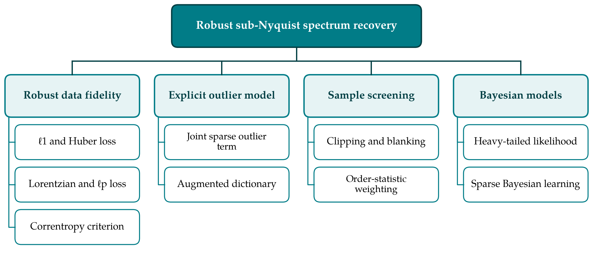
Figure 1: Families of methods for sparse spectrum recovery from sub-Nyquist samples under impulsive noise

5.1. Robust data-fidelity terms

The most direct change is to replace the squared residual with a function that grows more slowly. The ℓ1 norm of the residual gives least absolute deviations, the maximum-likelihood criterion for Laplacian noise, and combined with an ℓ1 penalty on the unknown it leads to a problem that is still convex and can be solved by linear programming or by splitting methods. The loss of Huber (1964) is quadratic for small residuals and linear for large ones, keeping efficiency under Gaussian background noise while bounding the influence of any one sample. Both fit the alternating direction method of multipliers, where the robust loss adds only a simple proximal step (Boyd et al., 2011).

Convex losses bound the influence of an outlier but do not remove it. Redescending losses go further. Carrillo et al. (2010) based a family of sampling and reconstruction methods on the Lorentzian norm, which arises from the Cauchy distribution and grows only logarithmically, so that a very large residual has almost no pull on the estimate. Residual norms with an exponent below one behave similarly and mirror, on the data side, the nonconvex penalties used to promote sparsity. The correntropy criterion of Liu et al. (2007) measures similarity through a Gaussian kernel and yields another bounded loss with a tunable width. The price in every case is a nonconvex objective. Convergence is to a stationary point, the result depends on initialisation, and the scale parameter that separates ordinary from outlying residuals has to be estimated from the data.

5.2. Explicit sparse-outlier models

A second family treats the impulses as an unknown to be estimated. The measurement is written as the sensing matrix applied to the sparse spectrum, plus a sparse error vector, plus small dense noise, and both sparse vectors are recovered together. The idea goes back to the error-correction setting of Candès and Tao (2005), where a codeword is decoded by linear programming despite gross errors in a fraction of its entries. Laska et al. (2009) applied it to compressive measurements under the name of justice pursuit, recovering signal and corruption from an augmented system formed by appending an identity matrix to the sensing matrix.

The appeal of this formulation is that it stays within standard compressed sensing. Any solver for sparse recovery can be run on the augmented matrix, and the theory asks only that the augmented matrix behave well on vectors sparse in both parts. Studer et al. (2012) gave recovery conditions in terms of the coherence between the signal dictionary and the dictionary in which the corruption is sparse. Those conditions expose a difficulty specific to spectrum sensing. Impulses are sparse in time, narrowband occupants are sparse in frequency, and the two bases are maximally incoherent, which is favourable; yet a sub-Nyquist front end has already mixed the time samples, so the corruption seen by the solver is sparse only if the acquisition preserves its localisation. Multicoset sampling does. The integrating and filtering stages of the other architectures smear an impulse across several outputs.

5.3. Screening before recovery

The oldest remedy for impulses in receivers is to clip or blank samples whose magnitude exceeds a threshold, and it carries over to compressive receivers with one caution. A blanked sample is a missing measurement, so the sensing matrix loses a row and the remaining rows must still support recovery. With random sampling patterns the loss of a few rows is tolerable and the theory of compressed sensing degrades gracefully. Threshold choice is the weak point. It is usually tied to a robust scale estimate such as the median absolute deviation, and weighted variants replace the hard decision with weights that fall as the residual grows, which turns screening into one step of an iteratively reweighted robust fit. Screening costs almost nothing and is therefore attractive as a first stage ahead of any of the other methods.

5.4. Bayesian formulations

Sparse Bayesian learning places a zero-mean Gaussian prior with its own variance on each unknown coefficient and estimates the variances from the data, most of which shrink to zero (Wipf and Rao, 2004). Robust versions change the likelihood. A Student-t noise model, written as a Gaussian whose precision varies from sample to sample under a Gamma prior, lets the algorithm learn which measurements are unreliable and discount them. The outlier-vector formulation fits the same machinery if the corruption is given its own sparsity-promoting prior. Bayesian methods estimate the noise scale and sparsity level along with the signal, which removes the tuning burden that troubles the redescending losses, and they return posterior variances that a spectrum-sensing decision rule can use. Their cost per iteration is the obstacle for long records and wide bands.

6. Gaps and Directions for Further Work

Four gaps stand out. The first concerns theory. Most robust recovery guarantees are proved for sensing matrices with independent random entries, while sub-Nyquist receivers produce structured matrices and, for multiband signals, jointly sparse unknowns. Results that hold for partial Fourier and sign-modulated matrices under heavy-tailed noise are scarce, and for α-stable noise even the right error metric is open to debate because second moments do not exist.

The second gap lies between the noise model and the hardware. Analyses place the impulse after acquisition, as an additive term on the digital measurements. A physical impulse arrives at the antenna, passes through mixers and filters that may saturate, and reaches the converter as a waveform shaped by the front end. Whether it remains sparse, and in which domain, depends on the architecture, and saturation makes the corruption signal-dependent. Joint modelling of front-end nonlinearity and impulsive interference has received little attention.

Third, sensing is a detection problem. The user of a spectrum sensor wants to know which bands are occupied, with controlled false-alarm probability, and not the best reconstruction of the waveform. Robust recovery papers mostly report reconstruction error. Detection thresholds that remain valid under heavy tails, and methods that estimate the support directly from robust covariance statistics, deserve more work. The fourth gap is practical: there is no agreed set of test conditions. Studies differ in the impulse model, its parameters and how the signal-to-noise ratio is defined when the noise variance is infinite, so that published comparisons are hard to reconcile. A shared, openly documented set of scenarios would allow methods to be compared on equal terms.

7. Conclusion

Sub-Nyquist spectrum sensing and robust estimation grew up separately, and the work reviewed here shows that they combine without great difficulty at the level of algorithms. A robust loss, an explicit outlier term, a screening stage or a heavy-tailed likelihood can each be attached to the standard sparse recovery model, and each protects against impulses under the noise model it assumes. What the literature does not yet provide is the same confidence at the level of systems: guarantees for the structured matrices that real receivers implement, models that follow an impulse through the analogue front end, and comparisons made under common conditions. Progress on those points would turn a collection of promising algorithms into design guidance for receivers that have to work in electrically noisy places.

Conflict of interest

To be declared by the author(s) before publication.

Funding

To be declared by the author(s) before publication.

References

[1] Blumensath, T. and Davies, M.E. Iterative hard thresholding for compressed sensing. Applied and Computational Harmonic Analysis https://doi.org/10.1016/j.acha.2009.04.002 27(3), 265-274 (2009).
[2] Boyd, S., Parikh, N., Chu, E., Peleato, B. and Eckstein, J. Distributed optimization and statistical learning via the alternating direction method of multipliers. Foundations and Trends in Machine Learning https://doi.org/10.1561/2200000016 3(1), 1-122 (2011).
[3] Candès, E.J. and Tao, T. Decoding by linear programming. IEEE Transactions on Information Theory https://doi.org/10.1109/TIT.2005.858979 51(12), 4203-4215 (2005).
[4] Candès, E.J., Romberg, J. and Tao, T. Robust uncertainty principles: Exact signal reconstruction from highly incomplete frequency information. IEEE Transactions on Information Theory https://doi.org/10.1109/TIT.2005.862083 52(2), 489-509 (2006).
[5] Carrillo, R.E., Barner, K.E. and Aysal, T.C. Robust sampling and reconstruction methods for sparse signals in the presence of impulsive noise. IEEE Journal of Selected Topics in Signal Processing 4(2), 392-408 (2010).
[6] Chen, S.S., Donoho, D.L. and Saunders, M.A. Atomic decomposition by basis pursuit. SIAM Journal on Scientific Computing https://doi.org/10.1137/S1064827596304010 20(1), 33-61 (1998).
[7] Donoho, D.L. Compressed sensing. IEEE Transactions on Information Theory https://doi.org/10.1109/TIT.2006.871582 52(4), 1289-1306 (2006).
[8] Feng, P. and Bresler, Y. Spectrum-blind minimum-rate sampling and reconstruction of multiband signals. Proceedings of the IEEE International Conference on Acoustics, Speech, and Signal Processing 1688-1691 (1996).
[9] Foucart, S. and Rauhut, H. A Mathematical Introduction to Compressive Sensing. Birkhäuser, New York (2013).
[10] Haykin, S. Cognitive radio: Brain-empowered wireless communications. IEEE Journal on Selected Areas in Communications https://doi.org/10.1109/JSAC.2004.839380 23(2), 201-220 (2005).
[11] Huber, P.J. Robust estimation of a location parameter. The Annals of Mathematical Statistics https://doi.org/10.1214/aoms/1177703732 35(1), 73-101 (1964).
[12] Landau, H.J. Necessary density conditions for sampling and interpolation of certain entire functions. Acta Mathematica https://doi.org/10.1007/BF02395039 117, 37-52 (1967).
[13] Laska, J.N., Davenport, M.A. and Baraniuk, R.G. Exact signal recovery from sparsely corrupted measurements through the pursuit of justice. Conference Record of the Forty-Third Asilomar Conference on Signals, Systems and Computers 1556-1560 (2009).
[14] Liu, W., Pokharel, P.P. and Príncipe, J.C. Correntropy: Properties and applications in non-Gaussian signal processing. IEEE Transactions on Signal Processing https://doi.org/10.1109/TSP.2007.896065 55(11), 5286-5298 (2007).
[15] Middleton, D. Statistical-physical models of electromagnetic interference. IEEE Transactions on Electromagnetic Compatibility https://doi.org/10.1109/TEMC.1977.303527 EMC-19(3), 106-127 (1977).
[16] Mishali, M. and Eldar, Y.C. Blind multiband signal reconstruction: Compressed sensing for analog signals. IEEE Transactions on Signal Processing https://doi.org/10.1109/TSP.2009.2012791 57(3), 993-1009 (2009).
[17] Mishali, M. and Eldar, Y.C. From theory to practice: Sub-Nyquist sampling of sparse wideband analog signals. IEEE Journal of Selected Topics in Signal Processing https://doi.org/10.1109/JSTSP.2010.2042414 4(2), 375-391 (2010).
[18] Mishali, M. and Eldar, Y.C. Sub-Nyquist sampling. IEEE Signal Processing Magazine https://doi.org/10.1109/MSP.2011.942308 28(6), 98-124 (2011).
[19] Nikias, C.L. and Shao, M. Signal Processing with Alpha-Stable Distributions and Applications. Wiley, New York (1995).
[20] Studer, C., Kuppinger, P., Pope, G. and Bölcskei, H. Recovery of sparsely corrupted signals. IEEE Transactions on Information Theory 58(5), 3115-3130 (2012).
[21] Tian, Z. and Giannakis, G.B. Compressed sensing for wideband cognitive radios. Proceedings of the IEEE International Conference on Acoustics, Speech and Signal Processing, IV-1357-IV-1360 (2007).
[22] Tropp, J.A. and Gilbert, A.C. Signal recovery from random measurements via orthogonal matching pursuit. IEEE Transactions on Information Theory https://doi.org/10.1109/TIT.2007.909108 53(12), 4655-4666 (2007).
[23] Tropp, J.A., Laska, J.N., Duarte, M.F., Romberg, J.K. and Baraniuk, R.G. Beyond Nyquist: Efficient sampling of sparse bandlimited signals. IEEE Transactions on Information Theory https://doi.org/10.1109/TIT.2009.2034811 56(1), 520-544 (2010).
[24] Wipf, D.P. and Rao, B.D. Sparse Bayesian learning for basis selection. IEEE Transactions on Signal Processing https://doi.org/10.1109/TSP.2004.831016 52(8), 2153-2164 (2004).
[25] Zoubir, A.M., Koivunen, V., Chakhchoukh, Y. and Muma, M. Robust estimation in signal processing: A tutorial-style treatment of fundamental concepts. IEEE Signal Processing Magazine https://doi.org/10.1109/MSP.2012.2183773 29(4), 61-80 (2012).

Article metrics

0 total accesses since publication. 0 citing articles have been indexed to date.