1. Introduction
Fresh waters cover a very small part of the Earth's surface and hold a disproportionate share of its described species, and they are losing that diversity faster than most terrestrial systems (Dudgeon et al., 2006). Monitoring is the precondition for any response. In Europe the Water Framework Directive obliges member states to classify the ecological status of rivers and lakes from their fish, invertebrates, aquatic plants and algae (European Parliament and Council, 2000), and comparable duties exist elsewhere. The conventional tools, electrofishing, netting, kick sampling and microscopy, are slow, need taxonomic specialists and can damage what they measure.
Environmental DNA, usually shortened to eDNA, offers a different route. Organisms release DNA into the water in mucus, faeces, gametes and shed cells. Ficetola et al. (2008) showed that the American bullfrog could be detected in French ponds from water samples alone. Combining that idea with DNA barcoding (Hebert et al., 2003) and high-throughput sequencing gave metabarcoding, in which a marker shared by a whole group is amplified and all the variants in a sample are sequenced together (Taberlet et al., 2012).
The method has been reviewed several times from the standpoint of molecular ecology (Deiner et al., 2017; Taberlet et al., 2018). The present article takes the standpoint of a monitoring agency or field ecologist deciding how far to rely on it. It considers what metabarcoding does well, where its results can mislead, and which parts of the workflow most need agreed standards.
2. Scope and Approach
This is a narrative review of the published literature on eDNA metabarcoding of water samples from rivers, lakes and ponds, with emphasis on fish, amphibians and macroinvertebrates. Single-species assays based on quantitative PCR are mentioned only where they clarify a point about detection. The review does not follow a systematic search protocol and makes no claim to completeness. Sources were chosen because they introduced a method, tested a specific source of bias, compared metabarcoding with established surveys, or addressed its use in regulation.
3. From Water Sample to Species List
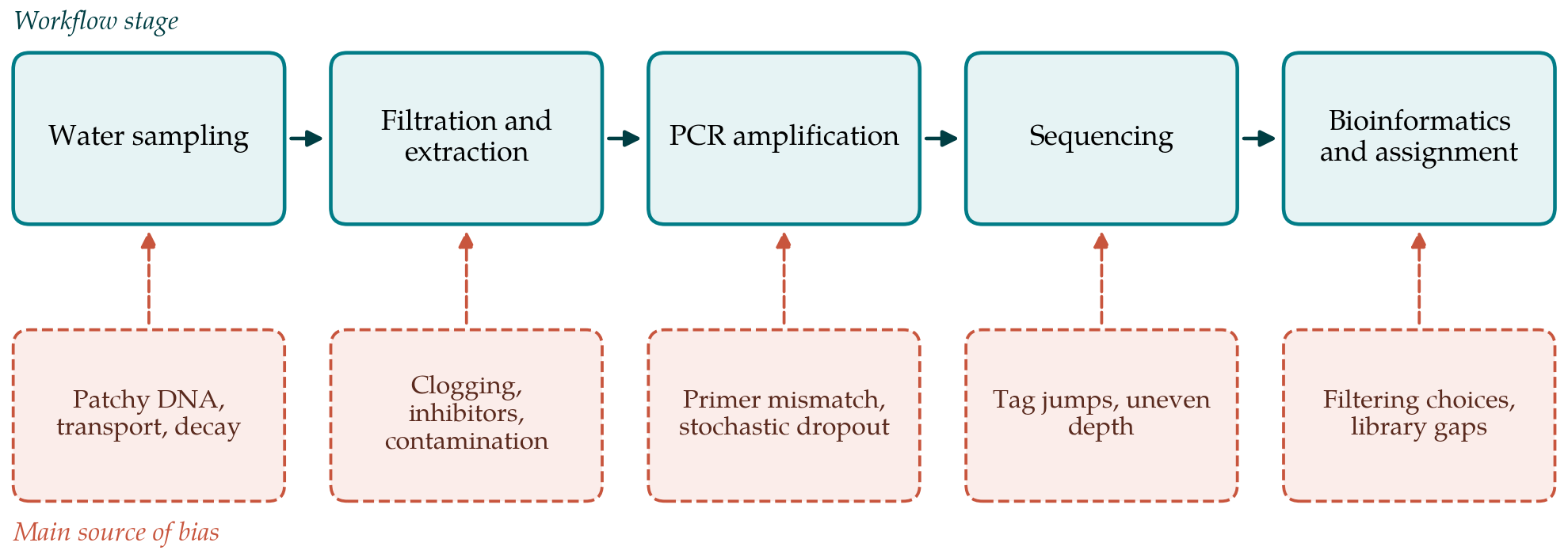
A metabarcoding survey has five stages, and decisions at each constrain what the final list can mean. Water is collected and its particulate matter captured, normally by filtration through a membrane or an enclosed capsule. DNA is extracted from the filter. A marker region is amplified by PCR with primers designed to match a target group, and sample-specific tags are attached. The pooled products are sequenced. Finally the reads are filtered, grouped and compared with a reference database to assign names (Taberlet et al., 2018).
The choice of marker defines the taxonomic window. For fish the most widely used primers target a short hypervariable stretch of the mitochondrial 12S ribosomal RNA gene, as in the MiFish set (Miya et al., 2015). For invertebrates the cytochrome c oxidase subunit I gene is preferred because it is the standard animal barcode and has by far the largest reference collection, though its variable primer sites make even amplification difficult. No single marker serves all groups, and surveys aiming at whole communities usually run two or more.
Bioinformatic practice has shifted from clustering reads into operational taxonomic units at a fixed similarity threshold towards inferring exact sequence variants with error models such as DADA2 (Callahan et al., 2016). Exact variants are reproducible labels that can be compared directly between studies, which clusters defined within one data set cannot. For monitoring, where results from different years and laboratories must be set side by side, that property matters a good deal.
4. Strengths
The first strength is sensitivity. In Danish ponds, lakes and streams, eDNA detected rare and threatened amphibians, fish, mammals, insects and crustaceans at most of the sites where they were known to occur (Thomsen et al., 2012). A large comparison across many sites found that metabarcoding recorded amphibian and fish species at least as often as traditional methods (Valentini et al., 2016). In Windermere, a lake with decades of fish survey data, eDNA metabarcoding recovered nearly all the species known from the lake, and the relative frequency of their sequences reflected their long-term rank abundance (Hänfling et al., 2016).
The second is that sampling is non-destructive. Collecting a few litres of water harms neither the organisms nor the habitat, which matters for protected species and for sites where electrofishing or netting is restricted. The third is breadth: one sample can be analysed for fish, amphibians, molluscs and insects with different primers, and the extract can be stored and analysed again when better markers or reference data appear.
A fourth strength is less often stated. Sequence data are an auditable record. A list produced by a field surveyor rests on that person's identifications, whereas raw reads can be deposited, reprocessed and reassigned by anyone. Field effort is also modest and needs little taxonomic training, which makes dense spatial coverage and volunteer sampling practical. The cost has not disappeared, however. It has moved from the riverbank to the laboratory and the reference library.
5. Sources of Bias
Each stage of the workflow introduces its own distortions. Figure 1 pairs the stages with the main bias arising at each, and Table 1 summarises the consequences for monitoring and the remedies in common use.
| Source of bias | Effect on results | Common remedy |
|---|---|---|
| Patchy distribution of DNA | Species present but missed | Several spatial replicates; larger volumes |
| Downstream transport | Detection away from the population | Interpret at reach or catchment scale |
| Decay and PCR inhibitors | False negatives | Rapid preservation; inhibition tests; internal controls |
| Contamination | False positives | Field, extraction and PCR blanks; one-way laboratory flow |
| Primer mismatch | Taxa missed; skewed read shares | In silico and mock community tests; multiple markers |
| Tag jumps and index hopping | Reads assigned to the wrong sample | Unique dual tags; thresholds set from blanks |
| Reference library gaps | Unassigned or misassigned reads | Curated regional libraries from vouchered specimens |
5.1. The ecology of eDNA
DNA in water is not the organism. Its concentration at a point depends on how much is shed, how it is transported and how quickly it decays, a set of processes that Barnes and Turner (2016) call the ecology of eDNA. In still water the signal can be highly local, so that a single shoreline sample misses species on the far side of a pond. In rivers it travels: Deiner et al. (2016) described rivers as conveyor belts of biodiversity information, with a sample integrating DNA from the catchment upstream. That is useful for an inventory of a catchment and awkward for a site-level assessment.
Persistence sets the time window. In experimental ponds and aquaria, DNA from bullfrog tadpoles and sturgeon became undetectable within about a month of removing the animals (Dejean et al., 2011). Decay is faster in warm water and is affected by acidity and sunlight, largely through their effects on microbial activity (Strickler et al., 2015). A positive result thus indicates recent presence somewhere within the water's reach. It does not prove a resident, living population, since DNA may also arrive in sewage, bait, bird faeces or resuspended sediment (Cristescu and Hebert, 2018).
5.2. Laboratory and sequencing biases
Amplification is the largest laboratory bias. Primers bind better to some templates than others, and the difference is multiplied through the cycles of PCR. Using mock communities of freshwater invertebrates, Elbrecht and Leese (2015) showed that read numbers varied by orders of magnitude among species present at equal biomass, and that some were not recovered at all. Read counts from a single marker therefore cannot be treated as estimates of abundance or biomass, and a species absent from the reads is not shown to be absent from the water.
Rare templates amplify erratically, so technical replicates of one extract often differ. Ficetola et al. (2015) examined how many PCR replicates are needed and how to treat detections that appear in only one of them, and recommended that replication be matched to the detection probability and analysed with site occupancy models. Sequencing adds further artefacts. Tags can recombine between amplicons during library preparation, placing reads in the wrong sample (Schnell et al., 2015). Blanks carried through every step are the only way to estimate such background, and thresholds for discarding low-count detections should be derived from them and reported.
5.3. Reference libraries and assignment
A sequence can be named only if a correctly identified reference exists. A gap analysis of barcode libraries for European aquatic biota found good coverage for fish and far poorer coverage for many invertebrate groups used in status assessment, with marked differences between countries (Weigand et al., 2019). Outside Europe and North America the gaps are wider, and in tropical rivers a large share of reads may match nothing at species level. Public databases also contain misidentified records. Curated regional libraries built from vouchered specimens are slow and unglamorous work, and nothing else substitutes for them.
6. Standardization Needs
Standardization does not require that every laboratory use the same kit. It requires that results be comparable and that their reliability can be judged. Goldberg et al. (2016) set out the minimum considerations for eDNA detection studies: explicit sampling design, contamination control in the field and laboratory, negative and positive controls at each stage, and full reporting of methods. Zinger et al. (2019) made a parallel case for metabarcoding, arguing that weak experimental design, with too few replicates and controls, undermines ecological conclusions however deep the sequencing.
For regulatory monitoring four areas need agreement. The first is field practice: volume filtered, number and placement of samples, filter type and preservation. The second is the laboratory: a fixed set of validated markers for each biological quality element, mock communities run alongside samples, and participation in ring tests between laboratories. The third is data: a defined pipeline or defined performance criteria, with raw reads and metadata archived. The fourth is interpretation. Existing biotic indices were calibrated on abundance data from nets and kick samples, and metabarcoding supplies, at best, presence and relative read frequency.
Two routes for the last problem are under discussion. One keeps the existing indices and feeds them presence data from DNA, accepting some loss of information. The other builds new indices directly from sequence data, including taxa never used in conventional assessment (Pawlowski et al., 2018). Hering et al. (2018) reviewed the options for the Water Framework Directive and judged that DNA-based identification could be taken up most readily for fish, with invertebrates and diatoms requiring further work on abundance and on intercalibration with the long-term record.
7. Gaps and Future Directions
Several questions remain open. The relation between read frequency and abundance holds in some systems, as in Windermere, and fails in mock community tests; when and why it holds is not well understood. Hydrological models that convert a detection into a probable source area are at an early stage. Most validation has been done in temperate lakes and streams, and large, turbid, tropical rivers with high sediment loads and poorly catalogued faunas present harder conditions for filtration and assignment alike.
There is also a question of continuity. Monitoring series are valuable because they are long, and replacing the method breaks the series. A period in which eDNA and conventional surveys are run side by side at the same sites is costly and is the only sound way to learn how the two relate. Until that overlap exists, metabarcoding is best used as a complement: for screening large numbers of sites, for detecting invasive or protected species early, and for groups that conventional methods sample poorly.
8. Conclusion
Environmental DNA metabarcoding has earned a place in freshwater monitoring. It is sensitive, harmless to the system sampled, broad in taxonomic reach and open to audit. It is also a chain of steps, each of which can add false negatives or false positives, and its output describes DNA in water, from which the presence of organisms must be inferred. The priorities are well understood: replication and controls reported as a matter of routine, validated markers, complete and curated reference libraries, archived raw data, and indices designed for the kind of information the method yields. With those in place, the technique can extend conventional surveys to more sites and more taxa than field teams could ever reach.
Conflict of interest
To be declared by the author(s) before publication.
Funding
To be declared by the author(s) before publication.