International Journal of Fluid Mechanics and Dynamics

Physics-Informed Neural Networks for Turbulence Closure: Progress, Pitfalls, and Benchmarking Needs

Andre Gopalakrishnan¹, Duc Souza², Jakub Lindo³

¹ Department of Mechanical Engineering, Achankovil Graduate Institute of Mechanical Engineering, Philippines, ² Department of Mechanical Engineering, Mekong School of Mechanical Engineering, Serbia, ³ Department of Mechanical Engineering, Balkan School of Mechanical Engineering, Czech Republic

Published 29 Jan 2026 Vol. 1, Article 2 10.62715/ijfmd.2026.v1.i1.pp7-12 0 accesses 0 citations

Download PDF XML HTML EPUB

0Accesses

0Citations

Abstract

The closure problem of turbulence, the need to model unresolved stresses in the averaged or filtered Navier-Stokes equations, has attracted machine learning since high-fidelity simulation data became plentiful. Physics-informed neural networks, which are trained by penalising the residual of the governing equations alongside any misfit to data, are one of several ways in which physical knowledge is being brought into learned closures. This narrative review separates three lines of work that share the label: constrained models embedded in a conventional solver, networks that act as solver and closure at once, and models trained through the solver. It summarises what each has demonstrated for Reynolds-averaged and large-eddy formulations and then turns to the difficulties that recur in the literature. These include stiff, multi-objective training, the bias of networks toward smooth solutions, the gap between accurate stresses and accurate mean flows, weak extrapolation beyond the training flows, and the cost of training relative to established solvers. The review argues that the field is held back less by a shortage of architectures than by the absence of agreed test cases, metrics and reporting practice, and it sets out what a credible benchmark suite for learned closures would have to contain.

Keywords: Machine learning Physics-informed neural networks Turbulence modelling Reynolds-averaged Navier-Stokes Large-eddy simulation Benchmarking

1. Introduction

Averaging or filtering the Navier-Stokes equations leaves a term, the Reynolds stress in the Reynolds-averaged (RANS) equations or the subgrid stress in large-eddy simulation (LES), that cannot be computed from the resolved field alone. Decades of modelling have produced closures of great practical value, from the one-equation and two-equation eddy-viscosity models described by Wilcox (2006) to the subgrid model of Smagorinsky (1963) and its dynamic successors. Their weaknesses are equally well known: separated flows, strong streamline curvature, secondary motions and transition are predicted poorly by models calibrated on simple shear flows.

The growth of direct numerical simulation databases prompted the question of whether closures could be learned instead of derived. The reviews by Duraisamy et al. (2019) and Brunton et al. (2020) chart the first wave of that effort. A recurring finding was that unconstrained regression performs badly, because a network free to violate invariance or conservation will do so as soon as it leaves its training data. Hence the interest in methods that carry physics inside the learning problem.

Physics-informed neural networks (PINNs), introduced in their current form by Raissi et al. (2019), are the best known of these methods, and the phrase has become a banner for a broader movement (Karniadakis et al., 2021). This review examines what the PINN idea has contributed to turbulence closure, where it has run into trouble, and what kind of evidence would allow claims in this area to be compared.

2. Scope and Terminology

This is a narrative review of the published literature, selective by design and concentrated on incompressible flow. A difficulty of terminology has to be settled first. In the strict sense a PINN is a network that represents the solution fields as functions of space and time and is trained by minimising the residuals of the governing equations, evaluated by automatic differentiation at collocation points, together with boundary and data terms. The idea of using a network as a trial solution of a differential equation is older than the name. In the turbulence literature, however, "physics-informed machine learning" was also adopted for something different: regression models for Reynolds-stress discrepancies whose inputs and outputs respect physical constraints (Wang et al., 2017). Both usages are covered here, and they are kept apart, because their strengths and failure modes differ.

3. Three Routes to a Physics-Informed Closure

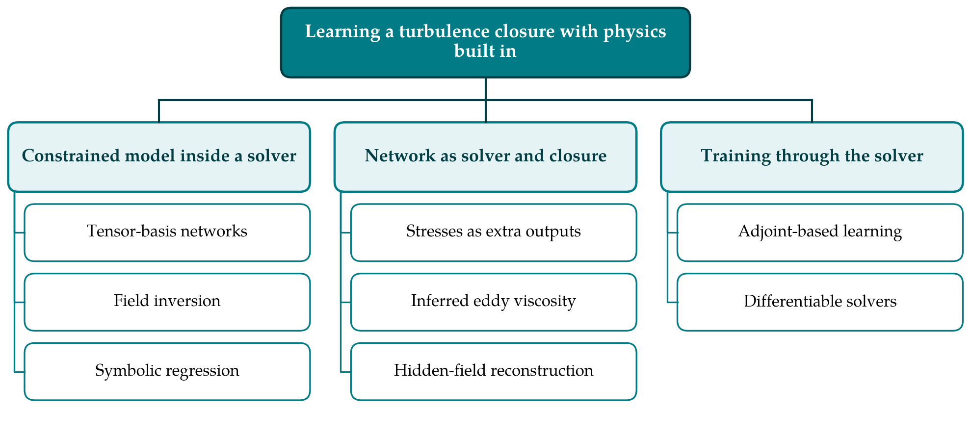
The work reviewed falls into three groups according to where the physics enters and where the closure lives. Figure 1 lays out the grouping, and the subsections below follow it.

Figure 1: Three routes by which physical knowledge enters a learned turbulence closure, with representative techniques

3.1. Constrained models embedded in a solver

The earliest successes kept the conventional solver and replaced or corrected its closure. The tensor-basis neural network of Ling et al. (2016) predicts the coefficients of the integrity basis derived by Pope (1975), so that the modelled anisotropy is Galilean and rotationally invariant by construction. Parish and Duraisamy (2016) proposed field inversion, in which a spatially varying correction to a baseline model is first inferred from data by solving an inverse problem and only then generalised by a learning algorithm. Others have used symbolic regression to obtain explicit algebraic stress relations that can be read and implemented like any other model. For LES, networks have been trained to return subgrid stresses or forces from filtered fields (Beck et al., 2019). None of these is a PINN in the strict sense. Physics enters through the choice of features, the form of the output and the solver that surrounds the model.

3.2. Networks that are solver and closure at once

In the strict PINN approach the mean or instantaneous fields are themselves network outputs. Jin et al. (2021) applied this to the incompressible Navier-Stokes equations, including turbulent channel flow, treating the network as a solver for a subdomain with boundary data supplied. Raissi et al. (2020) showed that velocity and pressure can be recovered from observations of a transported scalar by enforcing the equations as a constraint, a reconstruction task and not a predictive closure, but one that shows the value of the residual term when data are partial. Closest to the closure problem is the work of Eivazi et al. (2022), who solved the RANS equations with the Reynolds stresses as additional outputs, determined by the residuals and by data on the domain boundary, with no turbulence model assumed. The network there fits a closure for one flow. It does not yield a model that can be carried to another geometry, and that distinction is easily lost in summaries of the work.

3.3. Training through the solver

A third route accepts that a closure is only as good as the solution it produces and trains the model inside the solver. Sirignano et al. (2020) optimised a subgrid model with adjoint equations so that the filtered solution, and not the instantaneous stress, matches reference data. Kochkov et al. (2021) wrote the solver in a differentiable framework and learned corrections that let coarse grids reproduce fine-grid statistics in two-dimensional turbulence. These methods share with PINNs the use of automatic differentiation and of the governing equations as part of the training problem, and they avoid one of the central PINN weaknesses, since the discretised equations are satisfied exactly at every step instead of being a soft penalty. The survey of Karniadakis et al. (2021) places such hybrids of solver and network alongside PINNs within physics-informed learning.

4. Pitfalls

Enthusiasm for these methods has been tempered by a set of difficulties that appear again and again. Table 1 lists them with the sources that analyse each; the paragraphs below comment on those that bear most directly on closure.

Table 1: Recurring difficulties in physics-informed learning of turbulence closures and where they are analysed
Difficulty	How it shows up	Representative analysis
Unbalanced loss terms	Residual gradients swamp boundary and data terms; training stalls	Wang et al., 2021
Spectral bias	Smooth large scales are learned first; sharp gradients late or never	Rahaman et al., 2019; Wang et al., 2022
Hard optimisation landscape	Failure on convection-dominated problems despite adequate capacity	Krishnapriyan et al., 2021
Ill-conditioned stress closure	Small stress errors give large mean-velocity errors	Wu et al., 2019
A priori versus a posteriori	Good stress fit, unstable or inaccurate coupled simulation	Duraisamy et al., 2019
Narrow training set	Accuracy collapses on unseen geometry or Reynolds number	McConkey et al., 2021

The first three are properties of PINN training in general. The loss combines terms with different units and very different gradient magnitudes, and Wang et al. (2021) showed that the imbalance can prevent the boundary conditions from being learned at all. Analysis through the neural tangent kernel explains why components of the solution converge at widely separated rates (Wang et al., 2022), which is one face of the preference of networks for low frequencies documented by Rahaman et al. (2019). Krishnapriyan et al. (2021) demonstrated that the standard formulation can fail on simple convection and reaction problems, and that the cause is the optimisation landscape created by the soft constraint. Turbulent flows, with thin near-wall layers and a broad range of scales, exercise every one of these weaknesses, which is why published turbulent applications remain at modest Reynolds numbers and in simple geometries (Cai et al., 2021).

The fourth and fifth are specific to closure and more fundamental. Wu et al. (2019) showed that the RANS equations with an explicitly prescribed Reynolds stress can be ill-conditioned: even stresses taken directly from direct numerical simulation, with errors of a size no model could avoid, may yield mean velocities that are badly wrong. Treating part of the stress implicitly through an eddy viscosity restores conditioning. The lesson generalises. A model judged by how well it reproduces stresses on held-out snapshots, an a priori test, tells little about the flow it will produce once coupled to a solver. For LES the same gap appears as numerical instability when a network that correlates well with the true subgrid stress is inserted into a simulation (Beck et al., 2019).

Two further matters are raised less often than they should be. One is cost. A PINN that needs hours of training on a graphics processor to solve one steady RANS problem has to be compared with a finite-volume solver that reaches the same answer in minutes, and few papers report that comparison. The other is uncertainty. A learned closure applied outside its training range gives no warning that it is extrapolating, whereas the limits of the classical models, although real, are at least well mapped.

5. Benchmarking Needs

Progress in learned closures is hard to assess because studies seldom share test cases, baselines or metrics. Each paper tends to introduce its own flow, its own training split and its own measure of error, and to compare against a single conventional model run with unstated settings. Other areas of machine learning advanced quickly once common benchmarks existed, and turbulence modelling has a long tradition of validation cases on which to build.

5.1. Data and test cases

Suitable reference data already exist. The Johns Hopkins turbulence databases give open access to full space-time histories of canonical flows (Li et al., 2008). The flow over periodic hills, documented experimentally and numerically over a range of Reynolds numbers by Breuer et al. (2009), has become the customary test of separation and reattachment for learned RANS closures. McConkey et al. (2021) assembled a curated set of RANS solutions paired with high-fidelity labels across several geometries, built for training and testing closures. What is lacking is agreement on a tiered suite: canonical flows for sanity checks, a family of parametrically varied separated flows for interpolation, and geometrically distinct flows held out entirely to test extrapolation.

5.2. Metrics and reporting

A benchmark is defined as much by what is reported as by the flows it contains. Four requirements follow from the pitfalls above. Results should be a posteriori: mean velocity, skin friction, separation and reattachment locations from the coupled simulation, not stress correlations alone. Each learned model should be compared with at least two well-established closures run on the same grid, with settings disclosed. Training cost and inference cost should be stated next to the cost of the baseline solver. And the sensitivity of the result to random initialisation and to the weighting of loss terms should be shown, since PINN outcomes can vary markedly between nominally identical runs. Open-source PINN libraries now make it practical to publish the full training set-up alongside the paper.

6. Outlook

Several directions look productive. Hard enforcement of constraints, whether by building invariance into the architecture as the tensor-basis network does or by training through a solver that satisfies conservation exactly, has a better record than soft penalties for closure work. Hybrid schemes that use a PINN for what it does well, assimilating sparse measurements into a field consistent with the equations, and a conventional solver for prediction, play to the strengths of each. Interpretable outputs, algebraic expressions or corrections to named terms of an existing model, ease adoption because they can be inspected and implemented in production codes. The strict PINN as a general-purpose turbulent flow solver with an embedded closure remains, on present evidence, a research topic and not yet a competitor to established methods.

7. Conclusion

Physics-informed learning has changed how the closure problem is approached. It has produced invariant stress models, inversion-based corrections and solver-in-the-loop training, each with documented successes on separated and secondary flows that trouble classical closures. The strict PINN formulation has contributed most where data are sparse and the task is reconstruction, and least where a transferable predictive closure is wanted. Its training difficulties are now well characterised. What the field lacks is shared evidence. A tiered, open benchmark with a posteriori metrics, honest baselines and reported cost would do more to separate durable advances from fragile ones than another architecture.

Conflict of interest

To be declared by the author(s) before publication.

Funding

To be declared by the author(s) before publication.

References

[1] Beck, A., Flad, D. and Munz, C.-D. Deep neural networks for data-driven LES closure models. Journal of Computational Physics 398, 108910 (2019).
[2] Breuer, M., Peller, N., Rapp, C. and Manhart, M. Flow over periodic hills: Numerical and experimental study in a wide range of Reynolds numbers. Computers & Fluids 38(2), 433-457 (2009).
[3] Brunton, S.L., Noack, B.R. and Koumoutsakos, P. Machine learning for fluid mechanics. Annual Review of Fluid Mechanics https://doi.org/10.1146/annurev-fluid-010719-060214 52, 477-508 (2020).
[4] Cai, S., Mao, Z., Wang, Z., Yin, M. and Karniadakis, G.E. Physics-informed neural networks (PINNs) for fluid mechanics: A review. Acta Mechanica Sinica 37(12), 1727-1738 (2021).
[5] Duraisamy, K., Iaccarino, G. and Xiao, H. Turbulence modeling in the age of data. Annual Review of Fluid Mechanics https://doi.org/10.1146/annurev-fluid-010518-040547 51, 357-377 (2019).
[6] Eivazi, H., Tahani, M., Schlatter, P. and Vinuesa, R. Physics-informed neural networks for solving Reynolds-averaged Navier-Stokes equations. Physics of Fluids 34(7), 075117 (2022).
[7] Jin, X., Cai, S., Li, H. and Karniadakis, G.E. NSFnets (Navier-Stokes flow nets): Physics-informed neural networks for the incompressible Navier-Stokes equations. Journal of Computational Physics 426, 109951 (2021).
[8] Karniadakis, G.E., Kevrekidis, I.G., Lu, L., Perdikaris, P., Wang, S. and Yang, L. Physics-informed machine learning. Nature Reviews Physics https://doi.org/10.1038/s42254-021-00314-5 3(6), 422-440 (2021).
[9] Kochkov, D., Smith, J.A., Alieva, A., Wang, Q., Brenner, M.P. and Hoyer, S. Machine learning-accelerated computational fluid dynamics. Proceedings of the National Academy of Sciences 118(21), e2101784118 (2021).
[10] Krishnapriyan, A.S., Gholami, A., Zhe, S., Kirby, R.M. and Mahoney, M.W. Characterizing possible failure modes in physics-informed neural networks. Advances in Neural Information Processing Systems 34 (2021).
[11] Li, Y., Perlman, E., Wan, M., Yang, Y., Meneveau, C., Burns, R., Chen, S., Szalay, A. and Eyink, G. A public turbulence database cluster and applications to study Lagrangian evolution of velocity increments in turbulence. Journal of Turbulence 9, N31 (2008).
[12] Ling, J., Kurzawski, A. and Templeton, J. Reynolds averaged turbulence modelling using deep neural networks with embedded invariance. Journal of Fluid Mechanics https://doi.org/10.1017/jfm.2016.615 807, 155-166 (2016).
[13] McConkey, R., Yee, E. and Lien, F.-S. A curated dataset for data-driven turbulence modelling. Scientific Data 8, 255 (2021).
[14] Parish, E.J. and Duraisamy, K. A paradigm for data-driven predictive modeling using field inversion and machine learning. Journal of Computational Physics 305, 758-774 (2016).
[15] Pope, S.B. A more general effective-viscosity hypothesis. Journal of Fluid Mechanics 72(2), 331-340 (1975).
[16] Rahaman, N., Baratin, A., Arpit, D., Draxler, F., Lin, M., Hamprecht, F.A., Bengio, Y. and Courville, A. On the spectral bias of neural networks. Proceedings of the 36th International Conference on Machine Learning, PMLR 97: 5301-5310 (2019).
[17] Raissi, M., Perdikaris, P. and Karniadakis, G.E. Physics-informed neural networks: A deep learning framework for solving forward and inverse problems involving nonlinear partial differential equations. Journal of Computational Physics https://doi.org/10.1016/j.jcp.2018.10.045 378, 686-707 (2019).
[18] Raissi, M., Yazdani, A. and Karniadakis, G.E. Hidden fluid mechanics: Learning velocity and pressure fields from flow visualizations. Science https://doi.org/10.1126/science.aaw4741 367(6481), 1026-1030 (2020).
[19] Sirignano, J., MacArt, J.F. and Freund, J.B. DPM: A deep learning PDE augmentation method with application to large-eddy simulation. Journal of Computational Physics 423, 109811 (2020).
[20] Smagorinsky, J. General circulation experiments with the primitive equations: I. The basic experiment. Monthly Weather Review 91(3), 99-164 (1963).
[21] Wang, J.-X., Wu, J.-L. and Xiao, H. Physics-informed machine learning approach for reconstructing Reynolds stress modeling discrepancies based on DNS data. Physical Review Fluids 2(3), 034603 (2017).
[22] Wang, S., Teng, Y. and Perdikaris, P. Understanding and mitigating gradient flow pathologies in physics-informed neural networks. SIAM Journal on Scientific Computing 43(5), A3055-A3081 (2021).
[23] Wang, S., Yu, X. and Perdikaris, P. When and why PINNs fail to train: A neural tangent kernel perspective. Journal of Computational Physics 449, 110768 (2022).
[24] Wilcox, D.C. Turbulence Modeling for CFD, 3rd edition. DCW Industries, La Cañada, CA (2006).
[25] Wu, J., Xiao, H., Sun, R. and Wang, Q. Reynolds-averaged Navier-Stokes equations with explicit data-driven Reynolds stress closure can be ill-conditioned. Journal of Fluid Mechanics 869, 553-586 (2019).

Article metrics

0 total accesses since publication. 0 citing articles have been indexed to date.