1. Introduction
Automated microscopy has turned the cell-based screen from a single-readout assay into a high-dimensional measurement. Software such as CellProfiler segments every cell in every image and returns measurements of size, shape, intensity and texture for each stained compartment (Carpenter et al., 2006), and multiplexed staining protocols such as Cell Painting are designed to make that description as broad as possible (Bray et al., 2016). A screen of a compound library or a gene perturbation set therefore produces, for each treatment, not one number to be compared with control but a vector of several hundred to a few thousand.
Statistical practice has not kept pace with this change. Hit selection in screening grew up around single readouts and plate-quality measures such as the Z'-factor (Zhang et al., 1999), and although the case for formal inference in screening was made some time ago (Malo et al., 2006), the question of how to control error rates across treatments and features together is often handled by an arbitrary threshold or by a correction chosen for convenience. This article proposes a correction built on permutation of well labels. It describes the procedure and its rationale. It does not report an application to data, and its performance remains to be demonstrated.
2. Background
The design of the procedure follows from three observations about imaging screens and about the corrections usually applied to them.
2.1. The structure of an imaging screen
Cells are grown in multi-well plates. Each treatment occupies a small number of wells, commonly spread over replicate plates, and each plate carries a larger number of negative-control wells and some positive controls. Per-cell measurements are summarised to one value per feature per well, typically a median, and the well is the unit that received the treatment. The many cells within it are subsamples, not replicates (Lazic et al., 2018). Wells on one plate share reagents, incubation and imaging conditions, and systematic gradients across rows and columns are common, so normalisation against on-plate controls is a routine first step (Birmingham et al., 2009; Caicedo et al., 2017).
2.2. Why the usual corrections fit poorly
Testing every feature for every treatment creates a very large family of hypotheses. The Bonferroni correction and its step-down refinement by Holm (1979) control the probability of any false positive under arbitrary dependence, but they treat the tests as if each carried independent risk. Morphological features are far from independent: many are near-duplicates computed at different scales or in different channels. The effective number of tests is much smaller than the nominal number, and the correction is correspondingly too severe.
The false discovery rate procedure of Benjamini and Hochberg (1995) is less conservative and is the common alternative. Its guarantee was proved for independent tests and extended to a particular form of positive dependence, with a more stringent variant required for arbitrary dependence (Benjamini and Yekutieli, 2001). Feature sets contain both positive and negative correlations, so which case applies is unclear. Both families of correction also take the unadjusted p-values as given. With two to four wells per treatment and feature distributions that are often skewed or heavy-tailed, p-values from the t-distribution are unreliable in exactly the far tail where a stringent threshold operates.
2.3. Resampling-based adjustment
Permutation tests obtain the null distribution of a statistic from the data by recomputing it under relabellings that would be equally likely if the null hypothesis held (Good, 2005). Westfall and Young (1993) showed how to extend the idea to many tests at once: if whole observation vectors are relabelled, the joint distribution of all the test statistics is reproduced, correlation included, and the distribution of the largest statistic gives adjusted p-values that control the family-wise error rate. The method became standard in microarray analysis (Ge et al., 2003) and in neuroimaging, where the maximum statistic over an image of correlated voxels is the usual device (Nichols and Holmes, 2002). The imaging screen presents the same problem in a different layout, and the proposal below adapts the same solution to it.
3. The Proposed Procedure
The procedure has seven steps. Table 1 lists them with the assumption or safeguard attached to each, and Figure 1 shows the sequence. It takes as input a table of well-level feature values with plate, well position and treatment labels.
| Step | Action | Assumption or safeguard |
|---|---|---|
| 1. Unit and family | Take the well as the unit; declare which treatment-feature tests form the family | Family fixed before the data are examined |
| 2. Normalise | Scale each feature against negative controls on the same plate; remove positional trends | Wells on a plate comparable after correction |
| 3. Statistic | Compute a studentised difference from control for each treatment and feature | Statistics on a common scale across features |
| 4. Permute | Relabel whole wells at random within each plate, many times | Exchangeability within plates under the null |
| 5. Maximum | For each relabelling, keep the largest absolute statistic in the family | Feature vectors kept intact, so dependence is preserved |
| 6. Adjust | Compare each observed statistic with the distribution of maxima | Add-one estimator, so no p-value equals zero |
| 7. Check and report | Run held-out controls as mock treatments; document all settings | Mock treatments should not be called as hits |
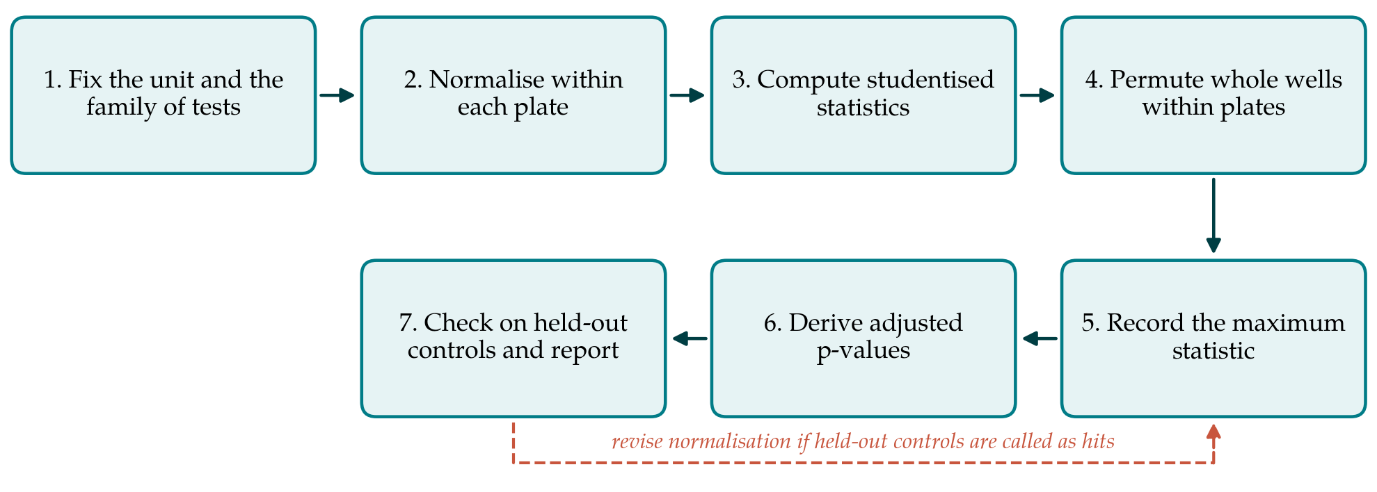
3.1. Step 1: Fix the unit and the family
The well is the experimental unit and all resampling is done on wells. The family of tests must be declared in advance, since the correction is only meaningful relative to it. Two choices are natural. If the aim is to say which features change under which treatment, the family is every treatment-feature pair. If the aim is only to find active treatments, each treatment can be given a single multivariate statistic and the family is the set of treatments. Redundant features may be removed beforehand to ease computation, although the correction does not require it.
3.2. Step 2: Normalise within plates
Each feature in each well is centred on the median of the negative-control wells on its plate and divided by their median absolute deviation. Where the controls reveal row, column or edge trends, these are estimated and removed. This step matters more here than in a parametric analysis, because the permutation in Step 4 treats wells on a plate as interchangeable, and uncorrected positional effects would break that assumption.
3.3. Step 3: Compute studentised statistics
For each treatment and feature the mean of the normalised replicate values is divided by an estimate of its standard error. Studentising is essential when a maximum is to be taken, since otherwise the features with the greatest variance dominate the reference distribution and the rest lose power. Because variance estimates from two or three wells are unstable, the standard error is better taken from the pooled spread of the control wells for that feature than from the treatment wells alone.
3.4. Step 4: Permute whole wells within plates
The labels that say which treatment or control each well received are shuffled among the wells of a plate, separately for each plate, and the statistics of Step 3 are recomputed for all tests. Two restrictions define the scheme. Shuffling is confined to plates, so that the plate acts as an exchangeability block in the sense used for permutation inference in the general linear model (Winkler et al., 2014). And a well keeps its entire feature vector when its label moves, so that every relabelled data set has the same correlation among features as the real one. Positive-control wells are excluded from the shuffle.
3.5. Step 5: Record the maximum statistic
From each relabelled data set only one number is kept: the largest absolute statistic across the whole family. The collection of these maxima, one per relabelling, estimates the distribution of the most extreme result that chance alone produces in a screen of this size, layout and correlation structure. Highly redundant features add little to the maximum, which is how the method adapts to the effective number of tests without that number ever being estimated.
3.6. Step 6: Derive adjusted p-values
The adjusted p-value of an observed statistic is the proportion of permutation maxima that equal or exceed it, computed with one added to both numerator and denominator so that it can never be zero (Phipson and Smyth, 2010). Tests whose adjusted p-value falls below the chosen level are declared hits, with the family-wise error rate controlled at that level. A step-down version, in which the maximum is taken over successively smaller sets of hypotheses ordered by their observed statistics, rejects at least as many hypotheses under the same guarantee (Westfall and Young, 1993).
3.7. Step 7: Check on held-out controls and report
Before the analysis, a portion of the negative-control wells on each plate is set aside and labelled as mock treatments with the same replicate layout as real ones. They pass through every step. Since they are known to be null, calls among them at a rate above the nominal level indicate that normalisation has left structure the permutation does not account for, and the analyst returns to Step 2. The report should state the family, the unit, the permutation scheme, the number of relabellings, the random seed, the software version and the outcome of this check.
4. Practical Considerations
The number of relabellings sets the smallest adjusted p-value that can be obtained, which is the reciprocal of that number plus one. Family-wise control at conventional levels therefore needs only a few thousand relabellings, far fewer than would be required to push unadjusted permutation p-values below a Bonferroni threshold. Where finer resolution in the tail is wanted, the upper tail of the maxima can be approximated by a generalised Pareto distribution (Knijnenburg et al., 2009). Each relabelling involves only means over small groups of wells, so the computation is matrix arithmetic and parallelises over relabellings.
A variant addresses a known weakness. Shuffling all wells assumes that no treatment has any effect, and in a screen with many active treatments the strongly perturbed wells are mixed into the reference distribution and widen it, which makes the procedure conservative. If plates carry enough negative controls, the reference distribution can instead be built from controls alone, by repeatedly drawing sets of control wells to stand in for each treatment at its plate locations. The variant assumes that an inactive treatment behaves like a control well, which is the working assumption of the screen itself. Investigators who prefer to control the false discovery rate can use the same relabellings to estimate it empirically, though the guarantee is then of a different kind.
5. Limitations and What Remains to Be Shown
The procedure is proposed and has not been validated in this article. Its guarantee rests on exchangeability of wells within a plate under the null hypothesis, and normalisation can only approximate that condition. Strong control of the family-wise error rate by the maximum-statistic method further requires that the joint distribution of statistics for the true null hypotheses does not depend on which other hypotheses are false, the condition Westfall and Young (1993) called subset pivotality. Compound effects on cell number, which alter the precision of every feature in a well, could violate it.
Three matters would need empirical study before the method could be recommended without reservation. The first is error control: whether, on plates containing only negative controls, the rate of false calls matches the nominal level across realistic plate layouts. The second is power relative to Holm and to false discovery rate procedures on data with known actives. The third is sensitivity to the normalisation method and to the number of control wells. Public image-based profiling data sets with annotated compounds would allow all three to be examined.
6. Conclusion
Multiple testing in imaging screens is a problem of dependence as much as of number. Relabelling whole wells within plates and referring each statistic to the distribution of the permutation maximum offers family-wise error control that uses the correlation among features instead of ignoring it, and that does not lean on distributional assumptions that a few replicate wells cannot support. The seven steps set out here make the assumptions explicit and include a check that can expose their failure. Whether the gain over standard corrections is large enough to justify the added computation is a question for empirical evaluation.
Conflict of interest
To be declared by the author(s) before publication.
Funding
To be declared by the author(s) before publication.