1. Introduction
Regulatory air quality monitoring was built around a small number of expensive, carefully maintained instruments. That model answers the question of whether a city meets a standard. It does not show how exposure varies from one street to the next. The arrival of inexpensive sensors prompted the suggestion that monitoring was undergoing a change of paradigm, in which dense networks operated by many kinds of user would supplement the reference stations (Snyder et al., 2013). For fine particulate matter, PM2.5, whose concentration near roads, kitchens and burning sites can differ sharply from the urban background, the attraction is plain.
The enthusiasm met an early warning. Lewis and Edwards (2016) argued that sensors were being sold and used without adequate validation, and an evaluation of commercial sensor platforms found that performance in the field fell short of what laboratory tests suggested and varied from unit to unit (Castell et al., 2017). The difficulty is acute for mapping. A map of a neighborhood compares sensors with one another, and the differences of interest are often of the same size as the errors of the devices. Unless every unit is tied to a common reference and kept tied to it, the map records the scatter of the instruments.
This article sets out a calibration procedure for small and medium-sized networks intended for neighborhood mapping of PM2.5. It is written for operators who have access to at least one reference-grade monitor, their own or an agency's. The procedure is a proposal built from the published literature. No network was calibrated for this article and no performance figures are claimed.
2. Background
A calibration can only correct errors whose causes are understood. This section summarises how the sensors work, where their errors arise and what approaches to correction have been published.
2.1. How the sensors measure and why they err
Nearly all low-cost particle sensors are optical. A small fan draws air past a laser or light-emitting diode, a photodiode records the light scattered by the particles, and firmware converts the signal to a mass concentration. The conversion embeds assumptions, because the light scattered by a particle depends on its size, shape and refractive index as well as its mass (Hinds, 1999). When the ambient aerosol differs from the one assumed, the reported mass is wrong. Evaluations against reference monitors show sensors that track reference concentrations closely over time yet differ in absolute level by an amount that changes with the source of the particles and becomes non-linear at high concentrations (Kelly et al., 2017; Zheng et al., 2018).
Humidity is the best characterised interference. Many atmospheric particles take up water as relative humidity rises, a behaviour that can be described with a single hygroscopicity parameter (Petters and Kreidenweis, 2007). Reference instruments dry or condition the sample. Low-cost sensors do not, so they see swollen particles and report too much mass, and in fog they may count droplets (Jayaratne et al., 2018). Crilley et al. (2018) showed that a correction based on this theory of water uptake greatly improved the agreement of a low-cost optical particle counter with reference data. Table 1 lists the principal sources of error and indicates where the procedure proposed here deals with each.
| Source of error | Effect on the reading | Treatment in the procedure | Source |
|---|---|---|---|
| Relative humidity | Particles take up water and scatter more light, so readings rise | Humidity term in the correction model (Stage 2) | Jayaratne et al., 2018 |
| Particle size and composition | Response differs between smoke, dust and mixed urban aerosol | Local collocation, repeated by season (Stages 1 and 4) | Kelly et al., 2017 |
| High concentration | Response departs from a straight line | Linearity check; segmented fit if needed (Stage 2) | Zheng et al., 2018 |
| Unit-to-unit variation | Units of one model give different readings side by side | Unit gain factors; outliers rejected (Stage 1) | Castell et al., 2017 |
| Ageing and drift | Response changes over months of exposure | Anchor and transfer units (Stage 4) | Malings et al., 2020 |
| Over-fitted correction | Output reflects the model more than the sensor | Simple model, held-out evaluation (Stage 2) | Hagler et al., 2018 |
2.2. Calibration approaches in the literature
The standard approach is collocation: the sensor is run beside a reference monitor and a statistical model is fitted that maps its output to the reference value. Models range from linear regression with a humidity term, as in the correction developed for one widely used sensor across the United States (Barkjohn et al., 2021), through regressions that add temperature and are evaluated over long deployments (Malings et al., 2020), to machine learning methods such as the random forest models applied to multi-pollutant sensor packages (Zimmerman et al., 2018). More flexible models usually fit the training period better. They also raise the concern voiced by Hagler et al. (2018), that a heavily adjusted value which draws on many external inputs may no longer be a measurement by the sensor at all.
A second family of methods calibrates sensors against one another once they are deployed, using moments when neighbouring nodes can be assumed to see the same air or passing a calibration from node to node; these blind, collaborative and transfer schemes are surveyed by Maag et al. (2018). Practical guidance on combining such elements has been assembled by Giordano et al. (2021), and the United States Environmental Protection Agency has published testing protocols and target values for PM2.5 sensors used in non-regulatory monitoring (U.S. EPA, 2021). The procedure below arranges these elements into a sequence suited to a mapping network.
3. The Proposed Procedure
The procedure has five stages that form a loop, since calibration is maintained and not completed. Figure 1 shows the loop, with the reference monitor at its centre as the fixed point to which every stage returns.
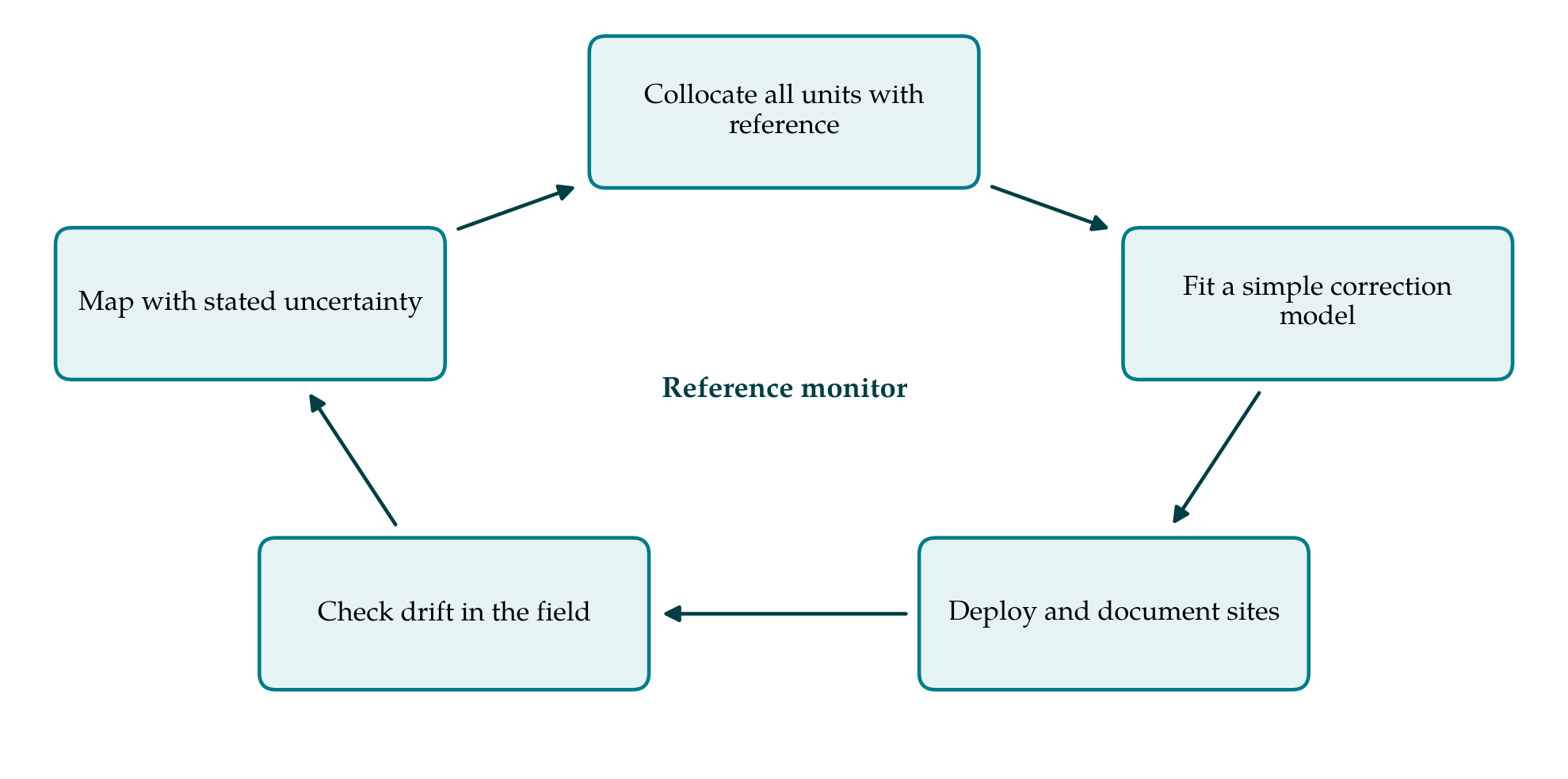
3.1. Stage 1: Collocate every unit before deployment
All sensors are installed together within a few metres of the reference monitor's inlet, in the enclosures and with the power and communications they will use in the field. The EPA protocol for base testing calls for at least three units run for at least thirty days (U.S. EPA, 2021); for a network the same period is applied to every unit. The period should include dry and humid conditions and the range of concentrations the network is expected to meet. Hourly averages are recorded from sensors and reference. Two outputs follow. The spread among units at each hour gives the precision of the batch, and any unit that departs persistently from the rest is set aside. The reference monitor's own uncertainty, which is not negligible at low concentrations, is noted so that the sensors are not asked to agree with it more closely than it agrees with itself.
3.2. Stage 2: Fit a simple, transparent correction
The starting model is linear in the sensor's reported PM2.5 with an additive term in relative humidity measured by the unit itself. A plot of residuals against concentration shows whether the response bends at the upper end, in which case a segmented fit is used above the break. One set of coefficients is estimated for the whole batch, and each unit then receives its own gain factor from its ratio to the batch median during collocation. This keeps the number of fitted quantities small and makes each one interpretable.
The model is judged on data it has not seen. Because hourly air quality data are strongly autocorrelated, the evaluation set should consist of whole blocks of days held out from fitting and not of hours drawn at random. Slope, intercept, coefficient of determination and root mean square error against the reference are reported and compared with the EPA target values. A machine learning model is adopted only if it is clearly better on the held-out blocks, and only with inputs measured at the sensor. Variables such as hour of day or concentrations from the reference station are excluded, because they would write the reference site's pattern onto every node and flatten the very gradients the network exists to find.
3.3. Stage 3: Deploy with documented siting
Each node is mounted at a consistent height with free air flow around the inlet, sheltered from direct rain and away from walls, vents and vegetation that would create a microenvironment. Where a node is deliberately placed near a source, such as a busy junction, that purpose is recorded. A siting sheet with coordinates, height, photographs in four directions and distances to nearby sources is kept for every node. One calibrated unit, the anchor, remains at the reference station for the life of the network.
3.4. Stage 4: Check for drift in operation
Three checks run in parallel. The anchor unit is compared with the reference continuously, and a sustained change in its corrected error signals that the model no longer fits the season or that the sensors are ageing. A transfer unit, freshly collocated, is carried around the network and left beside each node in turn for about a week, which gives a direct test of every node at its own site. And the network is screened as a whole: during regional episodes or calm night hours when concentrations are expected to be uniform, a node that stands apart from its neighbours is flagged. This third check is used only to trigger inspection. Automatic adjustment toward neighbours, as in blind calibration schemes (Maag et al., 2018), is avoided here because it risks removing real local differences. The whole batch is returned to the reference for collocation at least once in each distinct season.
3.5. Stage 5: Map with stated uncertainty
Corrected hourly data are aggregated to the averaging time appropriate to the question, usually daily or longer, since random error shrinks with averaging and bias does not. With a few tens of nodes the honest first product is a map of points. Surfaces can be interpolated by kriging, which also yields a prediction variance (Cressie, 1993), or estimated by land-use regression on road, land cover and population variables (Hoek et al., 2008). Either way the calibration error from Stage 2 and the transfer checks from Stage 4 set a floor: a difference between two sites smaller than that error should be reported as no detectable difference. Raw data, coefficients and the dates of every recalibration are published with the map.
4. Fitting the Procedure to Different Operators
The demands of the procedure fall mainly on access and patience. An agency with its own station can follow it as written. A university or community group needs an agreement to place sensors at an agency site, and such agreements are easier to obtain when the request is specific about duration, space and power. The month of collocation before deployment is the stage most often skipped, because it delays the visible start of a project, yet everything later depends on it. The statistical work requires only linear regression and can be done in a spreadsheet or in any free statistical package. A group without the capacity for the transfer-unit rounds can lengthen the interval between them, provided the anchor comparison is maintained.
5. Limitations and What Remains to Be Shown
The procedure has not been validated here. A field trial would need to show three things. First, that a correction fitted at one reference site holds at nodes elsewhere in the neighborhood, where the mix of particles may differ; the transfer-unit rounds test this only indirectly, and a second reference instrument moved among sites would test it directly. Second, that the simple model performs acceptably against the EPA targets across seasons in the climate concerned, since humidity corrections derived in one region have not always carried to another. Third, that the drift checks detect a failing sensor soon enough to protect the map.
Some limits are inherent in the devices. These sensors respond poorly to coarse particles, so the procedure applies to PM2.5 and not to dust-dominated PM10. No correction can recover information the sensor did not record, and a calibrated low-cost network remains a supplement to reference monitoring, suited to comparison and screening and not to judging compliance with standards.
6. Conclusion
A neighborhood map of particulate matter is a statement about differences between places, and it is only as good as the assurance that the sensors behind it would agree if they stood side by side. The five-stage procedure proposed here provides that assurance through a common reference, a correction simple enough to explain, and routine checks that the correction still holds. It asks for time at a reference station and for discipline in record keeping more than for equipment or expertise. Whether it delivers maps of sufficient accuracy for their intended use is a question for field trials, which the procedure is designed to make straightforward to conduct and to report.
Conflict of interest
To be declared by the author(s) before publication.
Funding
To be declared by the author(s) before publication.