1. Introduction
Since Kermack and McKendrick (1927) the standard description of an epidemic in a large population has been a system of ordinary differential equations for the numbers of susceptible, infective and removed individuals. Later models add latent, vaccinated, quarantined or age-structured classes, but they keep the same form, and the same qualitative features recur: solutions that start nonnegative stay nonnegative, the total population obeys a simple balance law, and a threshold quantity, the basic reproduction number, decides whether the infection dies out or persists (Hethcote, 2000; Brauer and Castillo-Chavez, 2012).
Outside a handful of special cases these systems are solved numerically, and the usual tools are the explicit Euler method and Runge-Kutta methods of higher order (Hairer et al., 1993). They are accurate when the step is small. When it is not, they can produce negative compartments, totals that drift when the scheme is modified to avoid them, and oscillations that have no counterpart in the model. The difficulty is practical: fitting a model to surveillance data or exploring a parameter space requires many thousands of integrations, some at parameter values that make the system stiff, and a failure of positivity in any one of them can corrupt the result without warning.
This article proposes a stepwise procedure for constructing finite difference schemes that preserve positivity, and the conservation law where there is one, for any step size. Each step is a known technique; what is offered is their arrangement into a routine that a modeller can apply to a new compartment model without specialist knowledge of numerical analysis. The procedure is described and illustrated on a single textbook model. It is not validated here by a programme of computations, and the closing sections say what such a validation would need to show.
2. Background
Three bodies of work supply the ingredients: the theory of positivity for standard methods, nonstandard finite difference schemes, and Patankar-type methods.
2.1. Why standard methods lose positivity
Consider the SIR model with births and deaths, written with standard incidence: S′ = Λ − βSI/N − μS, I′ = βSI/N − (γ + μ)I and R′ = γI − μR, where N = S + I + R. The explicit Euler method with step h multiplies S by the factor 1 − hβI/N − hμ before adding the recruitment term, and multiplies I by a factor containing −h(γ + μ). Positivity is guaranteed only if these factors are nonnegative, for which h(β + μ) ≤ 1 and h(γ + μ) ≤ 1 suffice. In models with fast processes, such as rapid progression through a latent class or high contact rates in a subgroup, the bound forces steps far smaller than accuracy alone would require.
Higher order does not remove the restriction. Bolley and Crouzeix (1978) showed that for a broad class of standard one-step and multistep methods, unconditional positivity is incompatible with order greater than one, and the theory of strong stability preserving methods expresses the admissible step of a Runge-Kutta scheme as a multiple of the Euler bound (Gottlieb et al., 2001). The implicit Euler method is unconditionally positive for problems of this type in exact arithmetic, but each step requires the solution of a nonlinear system, and the iteration used to solve it may itself leave the positive region. Discrete-time epidemic models built directly as difference equations show how badly a careless discretisation can behave, including period doubling and chaos that the differential equations exclude (Allen, 1994).
2.2. Nonstandard finite difference schemes
Mickens (1994) proposed building difference schemes by rules that depart from textbook practice in two main ways. The step h in the denominator of the discrete derivative is replaced by a function φ(h) that behaves like h for small steps, and nonlinear terms are evaluated at more than one time level, for example a product SI as S at the new level times I at the old one. The rules are reviewed in Mickens (2002), and Anguelov and Lubuma (2001) put them on a rigorous footing, defining a scheme as nonstandard when it uses either device and proving convergence and elementary stability results. The guiding idea is dynamic consistency: the discrete system should share the qualitative properties of the continuous one, such as positivity, invariants, equilibria and their stability, for all step sizes. Anguelov et al. (2014) applied the idea systematically to epidemiological models.
2.3. Patankar-type methods
A related device comes from computational fluid dynamics. Patankar (1980) treated sink terms by multiplying them by the ratio of the new value of the variable to the old one, which makes the update a division by a positive number and keeps the variable positive. Burchard et al. (2003) observed that the original trick destroys conservation, repaired it by weighting each production term in the same way as the destruction term it mirrors, and extended the construction to second order. For epidemic models the two traditions lead to closely related formulas, and the production and destruction language gives a convenient bookkeeping for the first steps of the procedure below.
3. The Proposed Procedure
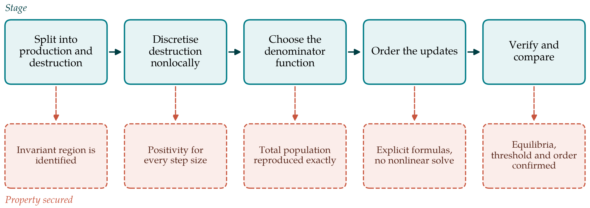
The procedure has seven steps. Figure 1 pairs the main stages with the property each is designed to secure, and the steps are described in turn using the SIR model above as a running illustration.
3.1. Step 1: Record the properties of the continuous model
Before any discretisation the modeller writes down what the scheme must reproduce: the invariant region, the equation satisfied by the total population, the equilibria, and the basic reproduction number, computed if necessary by the next generation method of van den Driessche and Watmough (2002). For the illustration, the nonnegative orthant is invariant, the total satisfies N′ = Λ − μN, there is a disease-free equilibrium with S = Λ/μ, and the reproduction number is β/(γ + μ).
3.2. Step 2: Split each equation into gains and losses
Each right-hand side is written as a sum of nonnegative production terms minus a sum of destruction terms, and every destruction term is checked to contain the variable of its own equation as a factor. This is the structural reason why solutions cannot cross zero, and it holds for compartment models by construction, since an outflow from a class is proportional to the number in it. Each transfer between compartments appears twice, once as a loss and once as a gain, and the pairs are noted.
3.3. Step 3: Discretise the losses nonlocally
In each equation the variable being depleted is taken at the new time level in every destruction term, and all other factors at the old level or at a level already computed. The gain that mirrors a loss is given exactly the same discrete form. Writing k for the time index, the susceptible equation becomes (Sk+1 − Sk)/φ = Λ − βSk+1Ik/Nk − μSk+1, the infective equation uses the same incidence term as a gain and (γ + μ)Ik+1 as its loss, and the removed equation has gain γIk+1 and loss μRk+1.
3.4. Step 4: Choose the denominator function
Adding the discrete equations gives a scheme for the total population, and the denominator function is chosen so that this scheme is exact. In the illustration the sum is (Nk+1 − Nk)/φ = Λ − μNk+1, and the choice φ(h) = (eμh − 1)/μ makes Nk coincide with the exact solution of the linear balance law at every grid point. When there is no demographic turnover the total is constant and φ(h) = h may be kept. For models in which the total does not satisfy a closed equation, Mickens (2007) gives a general recipe for constructing φ from the linear loss rates of the system.
3.5. Step 5: Order the updates so that they are explicit
Because each unknown appears linearly in its own equation, every update is solved by one division. The compartments are processed in the order in which infection moves through them, so that a value needed at the new level is already available. Here Sk+1 is the quotient of Sk + φΛ by 1 + φ(βIk/Nk + μ); Ik+1 is the quotient of Ik(1 + φβSk+1/Nk) by 1 + φ(γ + μ); and Rk+1 is the quotient of Rk + φγIk+1 by 1 + φμ. Numerators and denominators are sums of nonnegative quantities, so positivity holds for every step size without further argument.
3.6. Step 6: Verify the discrete properties algebraically
The list from Step 1 is now checked against the scheme by hand or with a computer algebra system. Fixed points are found by setting new and old values equal; in the illustration they satisfy the same equations as the equilibria of the differential system. Linearising the infective update at the disease-free state gives the multiplier (1 + φβ)/(1 + φ(γ + μ)), which is below one exactly when β < γ + μ, so the discrete threshold coincides with the continuous one for every h. A scheme that fails a check is revised at Step 3, usually by moving a factor from one time level to the other.
3.7. Step 7: Check accuracy against a reference solver
Qualitative fidelity says nothing about the size of the error. The final step compares the scheme with a high-order adaptive method run at a tight tolerance, on a sequence of halved steps, to confirm the expected first-order convergence and to find the step at which the error becomes acceptable for the purpose in hand. Table 1 sets the resulting scheme beside the standard alternatives.
| Scheme | Positivity | Order | Cost per step |
|---|---|---|---|
| Explicit Euler | Only below a step bound set by the fastest rate | 1 | One evaluation of the right-hand side |
| Classical Runge-Kutta | Only below a step bound | 4 | Four evaluations |
| Implicit Euler | Unconditional if the nonlinear system is solved exactly | 1 | Nonlinear solve |
| Nonstandard scheme of Steps 1 to 6 | Unconditional by construction | 1 | One division per compartment |
| Modified Patankar-Runge-Kutta | Unconditional (Burchard et al., 2003) | 1 or 2 | Linear solve per stage |
4. Fitting the Procedure to Practice
Three matters arise when the procedure is taken beyond the illustration. The first is the form of the incidence. Mass action incidence, saturating incidence and several infective classes are handled in the same way, provided the susceptible factor is taken at the new level; a force of infection that depends on several compartments is simply evaluated at the old level. The second is model size. With many compartments the order of updates follows the flow of individuals, and where flows form a loop, as with waning immunity, one transfer in the loop is evaluated with its source at the old level in the gain and at the new level in the loss, at the cost of exact conservation, or a small linear system is solved as in the modified Patankar approach.
The third matter is accuracy. Schemes built this way are first-order accurate, and because the incidence term mixes two time levels, a large step can displace the timing and height of the epidemic peak. The scheme is therefore best seen as a safe default: it will not fail, and it is accurate enough for exploratory work and for daily time steps in many applications. Where sharp accuracy is needed, it can serve as the fallback inside an adaptive code, or be replaced by a second-order positive method of the kind described by Burchard et al. (2003). General accounts of how discrete dynamics relate to continuous ones are given by Stuart and Humphries (1996).
5. Limitations and What Remains to Be Shown
The procedure is proposed, not tested. The algebraic claims made for the SIR illustration can be verified by direct substitution, but nothing here establishes how the procedure performs across the range of models in current use. A validation would need to show, for models with latent classes, vaccination, vector transmission and age structure, that Steps 3 to 5 can always be completed, that the discrete threshold agrees with the reproduction number, and how the error at practical step sizes compares with that of standard adaptive solvers at equal cost.
Two cautions are structural. Preservation of local stability at the disease-free state does not by itself guarantee the correct global behaviour, and endemic equilibria of larger models can lose stability in a discretisation even when they are fixed points of it; each case needs its own check. And dynamic consistency is a statement about qualitative behaviour. A scheme can be positive, conservative and faithful to every equilibrium while being quantitatively poor on the transient, which is often the part of an epidemic curve that matters most.
6. Conclusion
Positivity and conservation in epidemic compartment models follow from the structure of the equations, and a difference scheme can inherit both for every step size if losses are discretised nonlocally, gains mirror them, and the denominator function is taken from the balance law for the total population. The seven-step procedure set out here turns those principles into a routine that ends with explicit update formulas and a list of verified properties. It draws entirely on established methods. Whether it is as convenient and reliable on large applied models as on the textbook case is a question for systematic computational study.
Conflict of interest
To be declared by the author(s) before publication.
Funding
To be declared by the author(s) before publication.