1. Introduction
The standard empirical question about entrepreneurship is who becomes an entrepreneur. It is answered with a regression of entry on personal characteristics, or with a hazard model of the time to entry. Both designs reduce a working life to one transition. They cannot distinguish the person who ran a business for two years between jobs from the person who has owned firms for three decades, or the founder who started straight from university from the one who started after redundancy at fifty.
Burton et al. (2016) argued that entrepreneurship should be studied as part of a career: a spell, or several spells, located among other spells of work, and understood by what came before and after. Taking that view seriously requires a method that keeps the trajectory whole. Sequence analysis does so. It represents each person's history as an ordered string of states, measures how different any two strings are, and uses those differences to find typical patterns. One study of self-employment careers has applied this approach to panel data and related the resulting patterns to career outcomes (Koch et al., 2021), yet the method remains unfamiliar to most entrepreneurship researchers.
This article offers a stepwise procedure for analysts who hold longitudinal survey data and wish to trace entrepreneurial career paths. It reports no analysis of its own. The procedure is assembled from the methodological literature and is proposed for use, not validated here.
2. Background
Sequence analysis entered the social sciences when Abbott borrowed alignment techniques from molecular biology to compare careers and other ordered social processes (Abbott, 1995). The key tool was optimal matching, which defines the distance between two sequences as the least costly set of insertions, deletions and substitutions needed to turn one into the other. A review at the end of the first decade of applications (Abbott and Tsay, 2000) drew sharp criticism, notably from Wu (2000), who objected that the costs had no clear social meaning and that the method was disconnected from models of the processes generating the data.
The response has been called a second wave (Aisenbrey and Fasang, 2010). It brought new dissimilarity measures designed to answer specific criticisms, better tools for validating typologies, ways of linking sequences to covariates, and accessible software, above all the TraMineR package for R (Gabadinho et al., 2011). A recent survey of the field records how far these developments have gone and what remains unsettled (Liao et al., 2022). The procedure below relies on this second-wave toolkit.
3. The Procedure
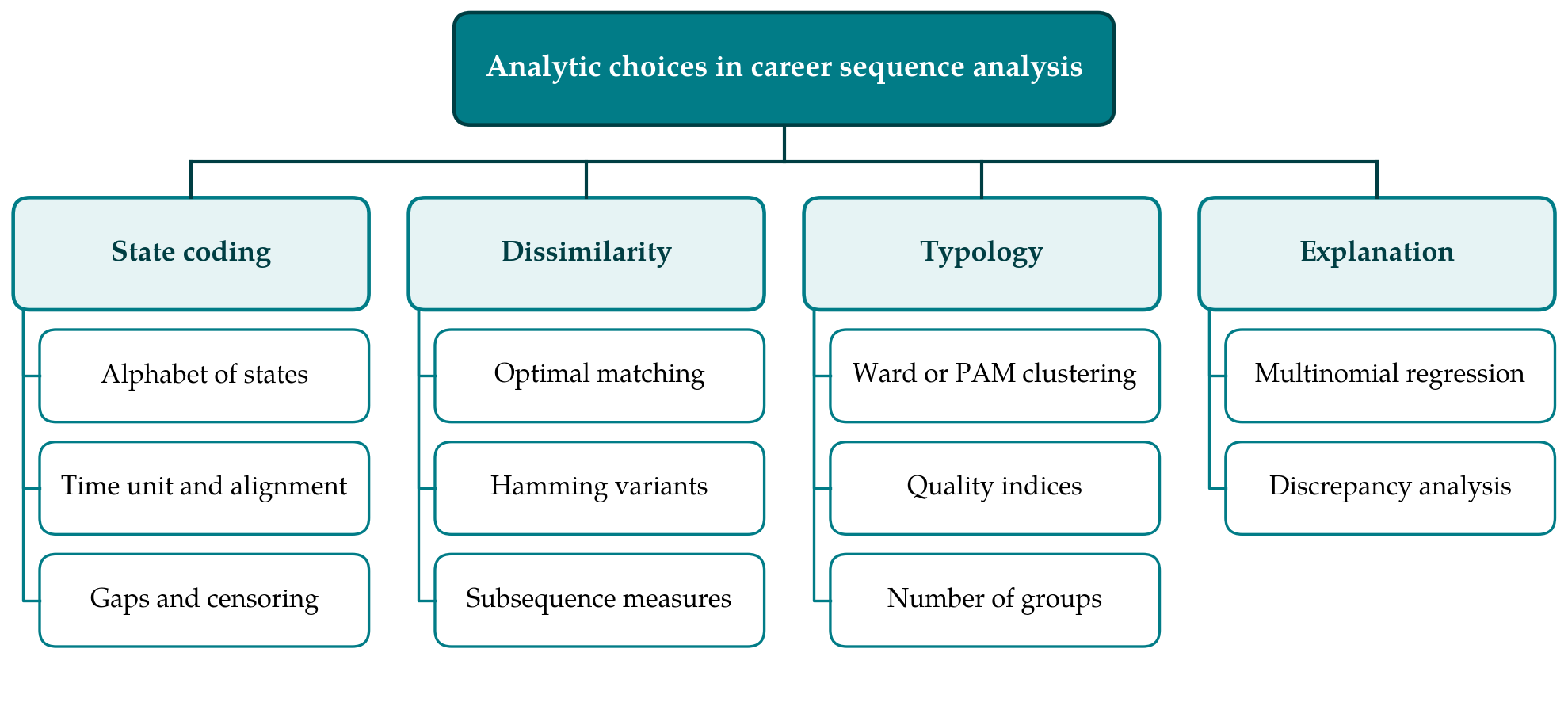
The procedure has six steps. Each involves decisions that affect the result, and Figure 1 groups those decisions under four headings. The steps are then taken in order.
3.1. Step 1: Define the states
The analyst first decides which states a person can occupy at each point in time. This alphabet embodies the research question. A minimal version distinguishes wage employment, self-employment, unemployment, education and inactivity. For entrepreneurship research it is usually worth splitting self-employment, for example into working alone and employing others, and adding a hybrid state for people who hold a wage job and run a business at once. Each additional state multiplies the number of distinct sequences and thins the data, so states that are rare or not relevant to the question should be merged. The alphabet and the rules for assigning ambiguous cases must be fixed and written down before any distances are computed.
3.2. Step 2: Build the sequences
Household panels such as the German Socio-Economic Panel (Goebel et al., 2019) record labour market status at each annual interview and often also in a monthly activity calendar covering the previous year. Either source can be turned into sequences. The analyst chooses the time unit, month or year, and the axis along which sequences are aligned. Aligning on age compares people at the same stage of life. Aligning on time since leaving education compares careers from a common start, which is usually the better choice for career questions. Sequences should cover a common window. Short gaps can be treated as a state in their own right or imputed from neighbouring states, while respondents with long gaps are better excluded, with the exclusions reported.
3.3. Step 3: Describe and visualise
Before any distances are computed the sequences should be looked at. Index plots draw each individual sequence as a horizontal line of coloured segments, and state distribution plots show the share of the sample in each state at each time point. Summary indicators for each sequence include the time spent in each state, the number of transitions, the within-sequence entropy and the turbulence measure of Elzinga and Liefbroer (2007), which increases with the number of distinct subsequences and decreases with the variance of spell lengths. These descriptions often answer simple questions directly, such as how common repeated spells of self-employment are, and they guard against a typology that reflects coding errors.
3.4. Step 4: Choose a dissimilarity measure
The choice of measure determines what counts as similar. Studer and Ritschard (2016) compare the available measures by their sensitivity to three aspects of a trajectory: the order in which states occur, the timing of states, and the time spent in each. Classic optimal matching with constant costs is a compromise among the three. Hamming distance, which permits only substitutions, is strict about timing, and the dynamic Hamming distance of Lesnard (2010) derives time-varying substitution costs from observed transition rates. Variants proposed by Halpin (2010) and Hollister (2009) adjust for spell duration and local context. Measures based on common subsequences stress order. Table 1 lists the main options and the kind of career question each suits.
| Measure | Most sensitive to | Suited to asking | Source |
|---|---|---|---|
| Optimal matching, constant costs | Duration, with some timing | How much of a career is spent in business ownership | Abbott and Tsay, 2000 |
| Optimal matching, transition-based costs | Duration | Which states substitute for one another in practice | Gabadinho et al., 2011 |
| Hamming distance | Timing | At what career stage self-employment occurs | Studer and Ritschard, 2016 |
| Dynamic Hamming distance | Timing | Whether entry coincides with typical transition ages | Lesnard, 2010 |
| Duration-adjusted and localized matching | Spells and context | Whether one long spell differs from many short ones | Halpin, 2010; Hollister, 2009 |
| Subsequence-based measures | Order | Whether employment precedes or follows founding | Elzinga and Liefbroer, 2007 |
No measure is correct in general. The analyst should state which aspect of the career matters for the question, choose accordingly, and repeat the analysis with at least one contrasting measure. If substitution costs are set by hand, the reasoning should be given, since it answers directly the criticism that costs are arbitrary.
3.5. Step 5: Build and validate a typology
The matrix of pairwise dissimilarities is passed to a clustering algorithm. Hierarchical clustering by the criterion of Ward (1963) and partitioning around medoids (Kaufman and Rousseeuw, 1990) are the usual choices, and the second can be started from the first. The number of clusters is chosen with the help of quality indices such as the average silhouette width, for which Kaufman and Rousseeuw suggest that values below about 0.25 indicate no substantial structure. Studer (2013) provides a practical guide to these indices and to clustering weighted survey data. Each cluster is then inspected with the plots from Step 3 and given a descriptive name, such as early and persistent ownership, late entry from employment, or brief episodes between jobs. Names are interpretations and should be offered as such.
3.6. Step 6: Relate sequences to covariates
Two routes lead from description to explanation. In the first, cluster membership becomes the outcome in a multinomial regression on characteristics fixed before the sequence begins, such as sex, parental self-employment and education, or a predictor of later outcomes such as earnings. This is simple but treats cluster assignment as if it were measured without error. The second route, discrepancy analysis, avoids clustering altogether: it partitions the total dissimilarity among sequences by a covariate, in the manner of an analysis of variance, and yields a pseudo R-squared with a permutation test (Studer et al., 2011). Used together, the two show whether an association depends on the typology chosen.
4. Fitting the Procedure to Panel Surveys
Survey data raise problems that textbook examples avoid. Panels lose respondents over time, and those who stay may differ from those who leave, for instance if business failure prompts a move and a missed interview. Requiring complete sequences therefore selects on stability, and longitudinal weights should be applied where the survey provides them. Careers under way when the panel began are censored on the left, and retrospective biography modules, where available, can fill the earlier years at the price of recall error. The window also has to be long enough for a career pattern to appear: ten or more years is a reasonable minimum, which restricts the analysis to mature panels.
Definitions need attention as well. Surveys identify self-employment by self-report, and the category mixes owners of incorporated firms, sole traders, freelancers and dependent contractors. Where the survey records whether the respondent has employees or whether the business is incorporated, that information should enter the alphabet. Self-employment as a secondary activity is recorded in some panels and not in others, and an analysis that ignores it will understate hybrid careers. All such decisions belong in a coding protocol published with the results, together with the software scripts.
5. Limitations and What Remains to Be Shown
Sequence analysis is descriptive. A typology summarises how careers differ and does not show why, and clustering algorithms return groups whether or not the data contain any. Results can shift with the alphabet, the time unit, the alignment, the cost scheme and the number of clusters, and readers have no way to judge robustness unless alternatives are reported. Because whole trajectories are the unit, the method also needs a completed window, so it says more about cohorts whose careers are well advanced than about recent entrants.
The procedure set out here has not been tested on entrepreneurial career data in this article. What remains to be shown is whether typologies of such careers are stable across measures and across national panels, whether they predict outcomes better than simpler summaries such as years of self-employment, and how they can be combined with event-history models that address causation. Those questions are empirical and are left to applications.
6. Conclusion
Entrepreneurial careers are sequences of states, and longitudinal surveys record them in a form that sequence analysis can use. The six-step procedure described here leads from the coding of states through the choice of a dissimilarity measure to a validated typology and its relation to covariates, and it asks the analyst to justify each decision along the way. Used with that discipline, the method can show patterns of entry, exit, return and combination that single-transition models leave out, and it gives the careers perspective on entrepreneurship an empirical instrument suited to its claims.
Conflict of interest
To be declared by the author(s) before publication.
Funding
To be declared by the author(s) before publication.