1. Introduction
Derivatives of non-integer order are almost as old as the calculus, but their systematic use in differential equations is recent. The monograph of Samko et al. (1993) fixed the operator theory, and the books of Podlubny (1999) and Kilbas et al. (2006) made it accessible to analysts working on differential equations. The appeal to modellers lies in memory: a fractional derivative at time t depends on the whole history of the function up to t, which suits viscoelastic materials, anomalous diffusion and other processes with hereditary behaviour (Caputo, 1967; Hilfer, 2000).
Nonlocal boundary conditions have a separate history. Il'in and Moiseev (1987) studied linear second-order problems in which the value at one end of the interval is tied to values at interior points, and nonlinear three-point problems for second-order equations followed within a few years. For evolution equations, Byszewski (1991) replaced the initial condition by a relation involving later times. Such conditions arise when a quantity cannot be measured at the boundary itself, or when the boundary responds to an average of the state. Combining them with fractional operators was a natural step, and from about 2005 onward papers on existence, uniqueness and, later, stability of solutions appeared in large numbers.
The size of that literature is itself an obstacle. Many papers differ only in the order of the equation, the type of derivative or the exact form of the boundary relation, and the shared method is easily lost among the variations. This article reviews the method. It describes the reduction to a fixed point problem, compares the theorems used to solve it, and separates the stability concepts that appear under one name. It is a narrative review of the published literature, organised by technique, and it states no result that is not already in print.
2. Scope and Approach
The review is confined to ordinary fractional differential equations on a bounded interval, mostly of order between one and two, with boundary conditions of multipoint or integral type. Partial differential equations, inclusions, impulsive problems and equations on unbounded domains are mentioned only where they clarify a point. The sources are the standard monographs, the survey of Agarwal et al. (2010), and papers that introduced a technique or are widely used as models. No attempt was made to count or classify all publications, and the selection reflects a judgement about which works shaped the methods now in use.
3. Preliminaries
Two definitions carry most of the theory. The Riemann-Liouville integral of order α > 0 of a function u on [0, 1] is the convolution of u with the kernel tα−1/Γ(α). The Riemann-Liouville derivative of order α, with n − 1 < α < n, is obtained by integrating to order n − α and then differentiating n times; the Caputo derivative reverses the order, differentiating first and integrating afterwards (Kilbas et al., 2006). The difference matters at the boundary. The kernel of the Riemann-Liouville derivative consists of the powers tα−1, ..., tα−n, some of which are singular at the origin, so natural conditions involve fractional integrals or weighted limits. The kernel of the Caputo derivative consists of ordinary polynomials of degree below n, and conditions on u(0) and u′(0) keep their classical meaning. This is the main reason the Caputo form dominates in applied work (Podlubny, 1999; Diethelm, 2010).
For initial value problems the basic theory is settled. Diethelm and Ford (2002) established the equivalence of the Caputo problem with a weakly singular Volterra equation together with dependence on the data, and Lakshmikantham and Vatsala (2008) developed fractional differential inequalities and comparison results. Boundary value problems borrow the same tools but lose the Volterra structure: the integral equation is of Fredholm type, so iteration no longer converges automatically and conditions on the size of the nonlinearity appear.
4. Reduction to a Fixed Point Problem
A model problem shows the pattern. Let 1 < α ≤ 2 and consider the Caputo equation Dαu(t) = f(t, u(t)) on [0, 1] with u(0) = 0 and u(1) = a u(ξ), where 0 < ξ < 1 and a is a real constant. Applying the fractional integral of order α to both sides gives u as the integral of f plus a polynomial of degree one with two free constants. The condition at zero removes one constant; the three-point condition determines the other, provided that aξ ≠ 1. Collecting terms, the solution is written as the integral over [0, 1] of G(t, s) f(s, u(s)), where G is an explicit Green function. Solutions of the boundary value problem are then the fixed points of the integral operator T defined by the right-hand side, acting on the space of continuous functions with the supremum norm.
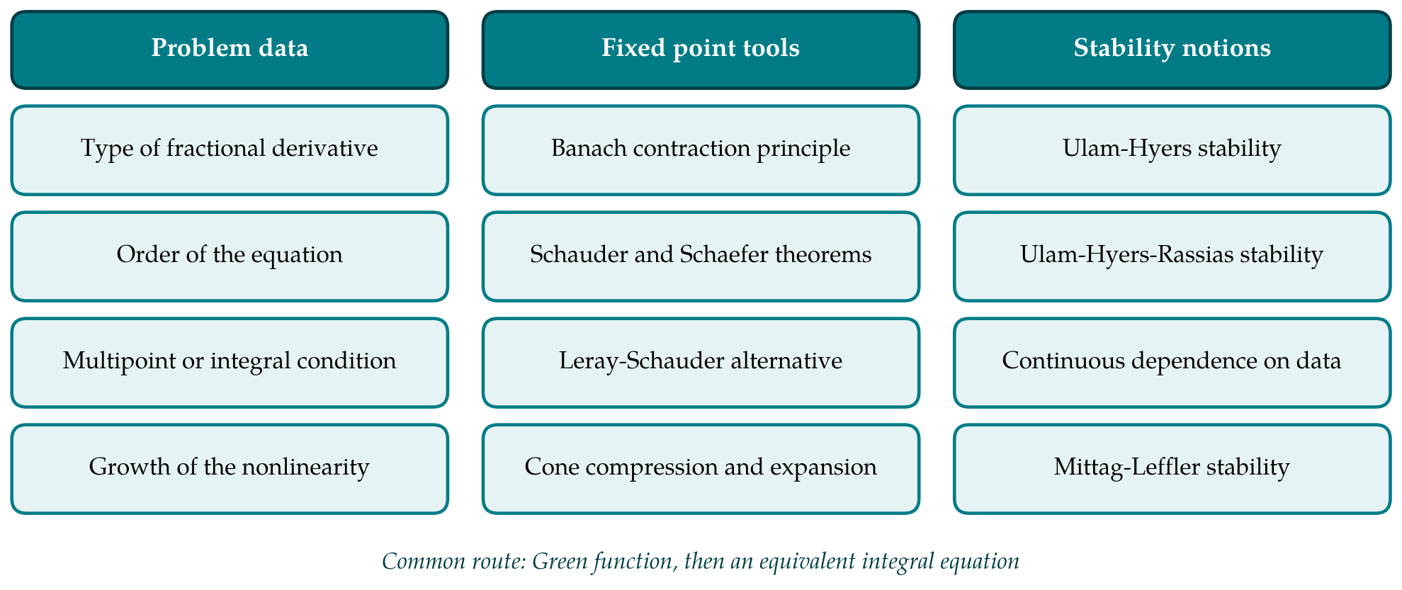
Every paper in the area carries out some version of this computation. With m interior points the scalar aξ is replaced by a sum, and with an integral condition by a Stieltjes integral, which contains the multipoint case as a special instance. For Riemann-Liouville equations of the form Dαu + f(t, u) = 0 with u(0) = 0, Bai and Lü (2005) derived the Green function for Dirichlet conditions and proved the positivity and the two-sided estimates on which later work depends, and Bai (2010) extended the analysis to a three-point condition. Benchohra et al. (2009) treated Caputo equations with nonlocal conditions of Byszewski type, and Ahmad and Nieto (2009) handled a coupled system with three-point conditions. Figure 1 places the ingredients side by side: the data of the problem, the fixed point theorem chosen, and the notion of stability examined afterwards.
Two technical points deserve attention. The first is the equivalence between the differential and integral formulations. It holds when f is continuous and the solution is sought in a class where the Caputo derivative exists and is continuous, but composition rules for fractional operators are not symmetric: integrating a derivative recovers the function only up to kernel terms, and the semigroup property known for integrals fails for derivatives in general (Diethelm, 2010). A proof that passes freely between the two forms should state the function class. The second point is compactness. The Green function contains the factor (t − s)α−1, which is continuous when α > 1 but weakly singular when the order, or the order of a lower term in the equation, is below one. Equicontinuity of the image of a bounded set then has to be checked by estimating increments of the kernel, after which the Arzelà-Ascoli theorem applies.
5. Existence and Uniqueness Results
Once the operator T is in hand, the choice of fixed point theorem is governed by what is assumed about f. Table 1 summarises the options. The hypotheses become weaker from the top of the table to the bottom, and so do the conclusions: uniqueness and a convergent iteration are available only under a Lipschitz condition.
| Theorem | Typical hypothesis on the nonlinearity | Conclusion | Representative source |
|---|---|---|---|
| Banach contraction principle | Lipschitz in the state, with constant small relative to the Green function | Unique solution; successive approximations converge | Benchohra et al., 2009 |
| Schauder theorem | Continuous and bounded, or sublinear growth | At least one solution in a closed ball | Ahmad and Nieto, 2009 |
| Schaefer theorem | Continuous, with an a priori bound on solutions of a one-parameter family | At least one solution | Benchohra et al., 2009 |
| Leray-Schauder nonlinear alternative | Growth controlled by a nondecreasing function of the norm | At least one solution in an open set | Granas and Dugundji, 2003 |
| Krasnosel'skii cone compression and expansion | Nonnegative, with sublinear or superlinear behaviour at zero and infinity | At least one positive solution | Bai and Lü, 2005 |
| Coincidence degree | Resonant linear part; sign or growth conditions | At least one solution at resonance | Mawhin, 1979 |
The contraction principle gives the cleanest statement. If f satisfies a Lipschitz condition in its second argument with constant L, and Λ denotes the supremum over t of the integral of |G(t, s)| in s, then T is a contraction whenever LΛ < 1. The constant Λ is explicit and depends on α and on the boundary data; it grows without bound as the nonlocal parameters approach the resonant configuration. The condition is restrictive, because on a Fredholm problem it cannot be relaxed by rescaling the norm in the way that works for Volterra equations, but it delivers uniqueness, a constructive scheme and, as discussed below, stability.
Topological theorems dispense with the Lipschitz condition at the cost of uniqueness. Schauder's theorem needs a closed, bounded, convex set mapped into itself, which is immediate when f is bounded and requires a growth restriction otherwise. Schaefer's theorem and the Leray-Schauder alternative replace the invariant set by an a priori bound on all solutions of the family u = λTu with 0 < λ < 1 (Granas and Dugundji, 2003). In practice the bound comes from a Gronwall inequality with a weakly singular kernel, or from a direct estimate using the growth function.
Positive solutions form a strand of their own, motivated by models in which the unknown is a concentration or a density. The method goes back to Krasnosel'skii (1964): one works in a cone of nonnegative functions that satisfy a Harnack-type lower bound inherited from the Green function, and shows that T compresses or expands the cone between two spheres. The estimates of Bai and Lü (2005) supply exactly the inequalities required. With nonlocal conditions the sign of the Green function is no longer automatic, and restrictions on the coefficients, such as 0 < aξα−1 < 1 in the Riemann-Liouville three-point problem, are imposed to keep it positive (Bai, 2010).
When the coefficients are resonant, in the model problem when aξ = 1, the linear operator has a nontrivial kernel and no Green function exists. The fixed point formulation is then replaced by the coincidence degree theory of Mawhin (1979), in which the linear part is a Fredholm operator of index zero and the nonlinearity is compact relative to it. The price is a set of sign or growth conditions on f that are harder to verify than a Lipschitz bound.
6. Stability of Solutions
The word stability is used in this literature in at least three senses, and results in one sense do not imply results in another.
6.1. Ulam-Hyers stability
The question of Ulam (1960) was whether a function that nearly satisfies a functional equation must lie near one that satisfies it exactly. Hyers (1941) answered it for the additive Cauchy equation in Banach spaces, and Rassias (1978) allowed the error to be unbounded. For differential equations, Rus (2010) formulated four related notions: an equation is Ulam-Hyers stable if there is a constant c such that every function whose residual in the equation is at most ε lies within cε of an exact solution; the generalised version replaces cε by a function of ε vanishing at zero; and the two Rassias versions weight the residual by a given function of t. Wang et al. (2011) carried these definitions over to Caputo equations and proved the first results by Gronwall-type estimates.
For boundary value problems solved by the contraction principle, Ulam-Hyers stability follows almost at once. If v has residual at most ε and satisfies the boundary conditions, then v differs from Tv by at most Λε in the supremum norm, and the standard estimate for contractions places v within Λε/(1 − LΛ) of the unique fixed point. Many published stability theorems for nonlocal problems are instances of this observation. The more demanding cases are those in which existence was obtained by a topological theorem, since without uniqueness the nearby exact solution has to be constructed, and those in which the approximate solution satisfies the boundary conditions only approximately.
6.2. Dependence on data and asymptotic notions
Continuous dependence asks how the solution changes when the order α, the nonlinearity or the boundary coefficients are perturbed. For initial value problems the answer is given by Diethelm and Ford (2002); for nonlocal boundary problems it reduces to the dependence of the Green function on its parameters and is uniform only away from resonance. This kind of result is what a modeller needs when the order of the derivative has been fitted to measurements and is known only approximately.
Asymptotic stability belongs to initial value problems on the half-line. Matignon (1996) showed that a linear fractional system of order α between zero and one is asymptotically stable when every eigenvalue λ of its matrix satisfies |arg λ| > απ/2, with algebraic and not exponential decay, and Li et al. (2009) introduced Mittag-Leffler stability and a Lyapunov direct method for nonlinear systems. These concepts have no direct counterpart on a bounded interval with two-sided conditions, and a paper on boundary value problems that announces a stability result should say which notion is meant.
7. Gaps and Directions for Further Work
Several questions are less settled than the volume of publications suggests. Sharpness is one: the contraction condition LΛ < 1 is sufficient, and little is known about how far it is from necessary for a given boundary configuration, or about the best constant in the Ulam-Hyers estimate. Resonant and near-resonant problems are another, since the Green function degenerates there and both existence and stability constants deteriorate. A third concerns the newer operators, including the interpolating derivative of Hilfer (2000) and derivatives taken with respect to another function, for which results are frequently obtained by transcription of the Caputo arguments, and it is not always clear what the generalisation adds.
There is also a gap between analysis and computation. Existence theorems proved by Schauder-type arguments are not constructive, and numerical methods for fractional boundary problems with nonlocal conditions are less developed than those for initial value problems (Diethelm, 2010). Ulam-Hyers estimates are well suited to closing this gap, because they convert a computable residual into an error bound, yet they are seldom used that way. Finally, the link to modelling is thin. Nonlocal conditions are routinely motivated by sensors placed inside a domain, but few studies start from a physical system and derive both the fractional order and the boundary relation from it.
8. Conclusion
Existence theory for fractional differential equations with nonlocal boundary conditions rests on a single construction: invert the linear part through a Green function and apply a fixed point theorem matched to the growth of the nonlinearity. Uniqueness and Ulam-Hyers stability come together under a Lipschitz condition that is small relative to the Green function, while topological and cone methods give existence, and positivity, under weaker assumptions. Read in this light, the literature is more unified than its size suggests. The questions that remain open concern sharp constants, resonance, constructive and numerical versions of the theorems, and a closer connection between the boundary conditions studied and the systems they are meant to describe.
Conflict of interest
To be declared by the author(s) before publication.
Funding
To be declared by the author(s) before publication.