1. Introduction
The method of Kaczmarz (1937) treats each equation of a linear system Ax = b as a hyperplane and projects the current iterate orthogonally onto one hyperplane after another. It was rediscovered in computed tomography as the algebraic reconstruction technique (Gordon et al., 1970) and has remained in use wherever the matrix is too large to factor and its rows can be accessed cheaply. For a sparse matrix the work of a step is proportional to the number of nonzeros in one row, and no storage beyond the iterate is needed.
For a long time the convergence rate of the cyclic method was hard to state, because it depends on the order of the rows. Strohmer and Vershynin (2009) showed that choosing the row at random, with probability proportional to its squared Euclidean norm, gives a simple bound on the expected error in terms of the matrix alone. This note is concerned with what the resulting theory implies when the system is ill-conditioned and sparse, the situation in which a row-action method is most tempting and its behaviour least intuitive.
2. The Basic Rate and Its Condition Number
For a consistent system with a matrix of full column rank, the Strohmer-Vershynin theorem states that the expected squared error contracts at every step by at least the factor 1 - (s / F)2, where s is the smallest singular value of A and F its Frobenius norm (Strohmer and Vershynin, 2009). The ratio F / s is a scaled condition number. Its square is never smaller than the number of unknowns n, with equality when all singular values coincide, and it is at most n times the square of the ordinary spectral condition number. A natural unit of work is therefore the sweep of n steps, and the number of sweeps needed for a fixed reduction of the error grows like the square of the scaled condition number divided by n.
Two comparisons put this in perspective. The method is one instance of the sketch-and-project family of Gower and Richtárik (2015), in which coordinate descent and block methods appear as other choices of the sketch, and within that family the dependence on the squared condition number is typical. The conjugate gradient method applied to the normal equations, in contrast, depends on the condition number of A to the first power (Saad, 2003), at the cost of a product with A and with its transpose in every iteration.
3. What Ill-Conditioning Does to the Iterates
The bound of the previous section is a worst case over all directions of the initial error. A sharper description was given by Steinerberger (2021): the expected component of the error along each right singular vector decays geometrically at a rate set by the square of the corresponding singular value relative to the squared Frobenius norm. Components along large singular vectors disappear within a few sweeps. Components along the small ones persist, and after an initial phase the error points predominantly in the directions that the matrix barely sees.
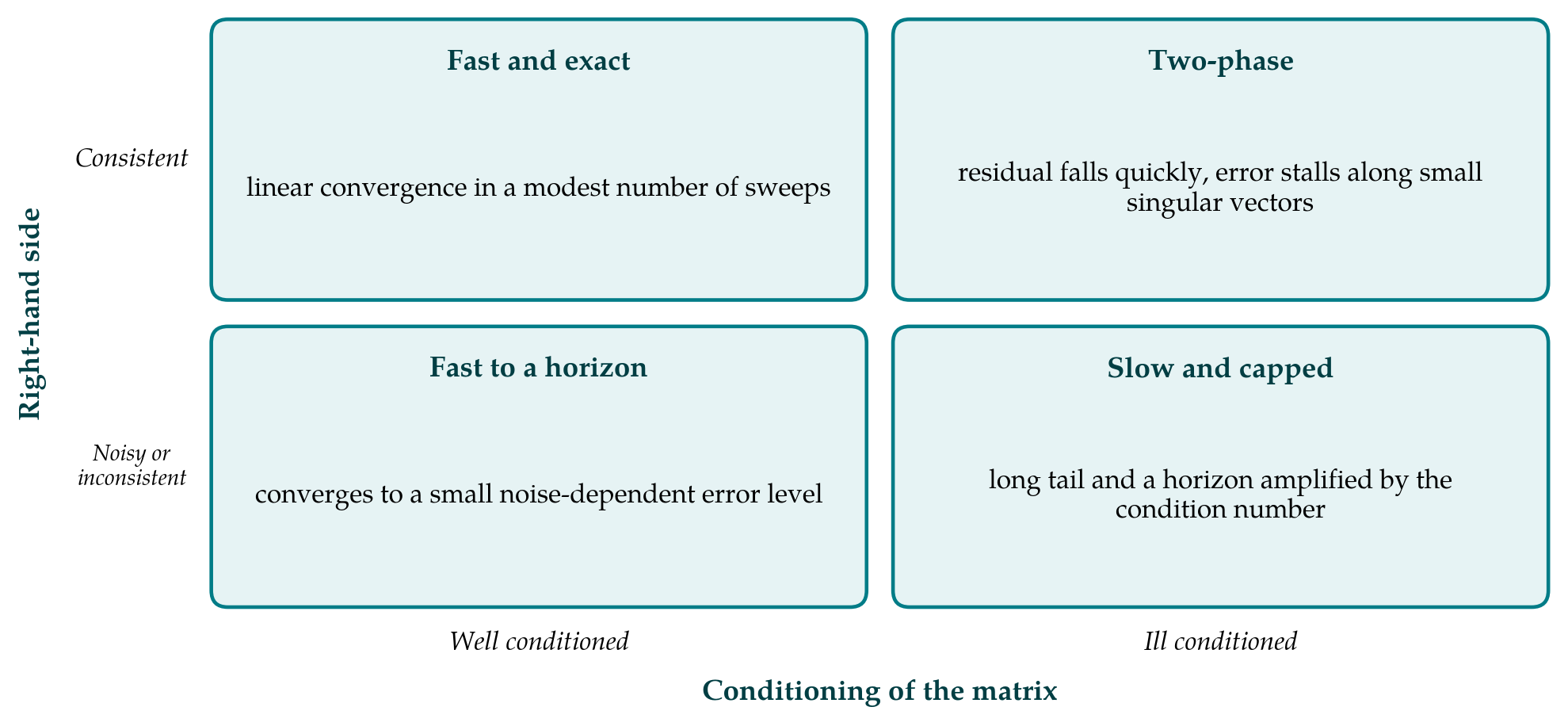
The practical consequence is a two-phase history. Early on, both the error and the residual drop quickly. Later the residual, which weights each error component by its singular value, continues to look small while the error is dominated by the slowly decaying components. A stopping test based on the residual alone can therefore end an ill-conditioned solve at an iterate that fits the equations well and is still far from the solution. In inverse problems, where those components carry the noise, the same effect acts as a regularizer when the iteration is stopped early. Figure 1 places this regime beside the three others that arise when conditioning and consistency of the right-hand side are varied together.
4. Noise and Inconsistency
Ill-conditioned systems in practice rarely have exact right-hand sides. Needell (2010) proved that, when each equation is perturbed, the randomized Kaczmarz iterates still converge linearly at the Strohmer-Vershynin rate, but only to within a fixed distance of the solution of the unperturbed system. That distance, often called the convergence horizon, is proportional to the scaled condition number times the largest perturbation of an equation relative to the norm of its row.
For inconsistent overdetermined systems the horizon can be removed. The randomized extended Kaczmarz method of Zouzias and Freris (2013) interleaves the row projections with column projections that progressively strip from the right-hand side its component outside the range of A, and converges in expectation to the minimum-norm least-squares solution. The rate again involves the square of the scaled condition number, so the extension cures inconsistency and not ill-conditioning. Table 1 summarizes how this and other variants bear on the difficulty.
| Variant | Idea | Bearing on ill-conditioning |
|---|---|---|
| Basic randomized (Strohmer and Vershynin, 2009) | Sample rows by squared norm, project | Rate set by squared scaled condition number |
| Extended (Zouzias and Freris, 2013) | Add column projections on the right-hand side | Removes the horizon; rate unchanged in kind |
| Block (Needell and Tropp, 2014) | Project onto several rows at once | Gains if rows split into well-conditioned blocks |
| Greedy (Bai and Wu, 2018) | Favour rows with large residual entries | Fewer steps; needs residual information |
| Accelerated (Liu and Wright, 2016) | Nesterov-type momentum on the iteration | Improves the dependence on the condition number |
5. The Role of Sparsity
Sparsity makes each step cheap, but the rate theorems above do not involve the sparsity pattern at all: the same singular values give the same expected contraction whether the matrix is dense or sparse. A sparse matrix whose scaled condition number is large, as for discretized differential or integral operators on fine grids, will need many sweeps.
Sparsity matters in two indirect ways. Rows with disjoint supports are orthogonal, so projections onto them commute and can be carried out simultaneously, which is the basis for parallel and block implementations. Needell and Tropp (2014) analyse block projections and show that the rate improves when the rows can be partitioned into blocks that are individually well conditioned, a partition that structured sparse matrices often admit. Sparsity also affects sampling: sampling by row norm is equivalent to uniform sampling after the rows have been normalized, so the weighting is a diagonal scaling of the system, and other scalings may serve a given matrix better (Censor et al., 2009).
6. Practical Remarks
Three recommendations follow from the results collected here. First, progress on an ill-conditioned system should not be judged by the residual alone; a bound on the smallest singular value, where one is available, converts the residual into an error estimate. Second, greedy selection (Bai and Wu, 2018) and acceleration (Liu and Wright, 2016) reduce the number of steps but need up-to-date residual entries or extra vectors and parameters. Third, when products with A and its transpose are affordable, a preconditioned Krylov method is normally the stronger choice for high accuracy (Saad, 2003). Randomized Kaczmarz keeps its place when rows arrive one at a time, when memory is the constraint, or when low accuracy suffices.
7. Conclusion
The published analysis of the randomized Kaczmarz method gives a consistent account of its behaviour on ill-conditioned systems. Convergence is linear in expectation, with a rate governed by the squared scaled condition number; error along small singular directions is the last to go; noise sets a floor that the same condition number raises; and sparsity changes the price of a step but not the number of steps. Users should expect a fast start and a long tail.
Conflict of interest
To be declared by the author(s) before publication.
Funding
To be declared by the author(s) before publication.