International Journal of Geotechnical and Seismic Engineering

Site Response Analysis for Deep Alluvial Basins Using Ambient Vibration Array Measurements: A Proposed Workflow

Linh Dang¹, Isha Carrington², Carmen Radovic³

¹ Department of Engineering, Nile Delta Institute for Advanced Engineering, Iceland, ² Department of Engineering, Lapland Academy of Engineering, Italy, ³ Department of Engineering, Thames University Centre for Engineering, Kazakhstan

Published 14 Jun 2026 Vol. 1, Article 3 10.62715/ijgse.2026.v1.i1.pp15-20 0 accesses 0 citations

Download PDF XML HTML EPUB

0Accesses

0Citations

Abstract

Site response analysis needs a shear wave velocity profile that reaches the seismic bedrock. In deep alluvial basins that horizon may lie several hundred metres below the surface, beyond the reach of routine boreholes and of active surface wave surveys with hammer or weight-drop sources. Arrays of seismometers recording ambient vibrations can recover surface wave dispersion at the long wavelengths required, at modest cost and without drilling, and the techniques for processing such records are mature. What practitioners often lack is an agreed route from the field records to the amplification functions used in design, with the uncertainty of the velocity model carried through. This article proposes such a workflow in seven steps: a desk study that fixes the target depth, acquisition with nested arrays and single stations, extraction of dispersion and horizontal-to-vertical spectral ratio curves, joint inversion to an ensemble of profiles, checks against independent information, one-dimensional site response analysis over the ensemble, and reporting. The purpose and the decisions involved in each step are explained with reference to published guidelines. The workflow is a proposal assembled from established methods. It has not been applied to a site or validated here, and the article states what a validation would need to show.

Keywords: Site response analysis Ambient vibration arrays Shear wave velocity Surface wave inversion Alluvial basin Microtremor

1. Introduction

The amplification of earthquake ground motion by soft sediments is controlled, to first order, by the variation of shear wave velocity with depth and by the impedance contrast at the base of the sediments. For a shallow site the profile can be measured down to rock by downhole or crosshole logging, or by active surface wave methods such as multichannel analysis of surface waves (Park et al., 1999). In a deep basin none of these is adequate on its own. Boreholes of the necessary depth are expensive, and active sources do not generate enough energy at the low frequencies whose wavelengths sample the deeper layers.

Ambient vibrations fill the gap. The ground is in constant motion from ocean waves, wind and human activity, and at frequencies below about one hertz this motion is dominated by surface waves of natural origin (Bonnefoy-Claudet et al., 2006). An array of sensors spread over hundreds of metres can measure the phase velocity of those waves as a function of frequency, and inversion of the resulting dispersion curve yields a velocity profile. The principle goes back to Aki (1957), and the practice has been codified in the guidelines that followed the InterPACIFIC blind comparisons (Foti et al., 2018).

This article sets out a workflow that links array measurements to site response analysis for a deep basin site. It is a methodology article. The procedure is proposed on the basis of the published literature and has not been applied or validated here; no measurements or computed results are presented. The emphasis is on the decisions an analyst must take and on keeping the non-uniqueness of the inversion visible in the final product.

2. Background

Three bodies of method are combined in the workflow: array processing of ambient noise, the single-station spectral ratio, and one-dimensional wave propagation analysis.

2.1. Array techniques

Two families of array technique are in common use. Frequency-wavenumber analysis treats the wavefield in each narrow frequency band as a sum of plane waves and searches for the velocity and direction that maximise the coherent power across the array; the high-resolution form introduced by Capon (1969) is the usual choice. Spatial autocorrelation, in Aki's formulation, relates the azimuthally averaged coherency between sensor pairs to a Bessel function of frequency, separation and phase velocity. The modified method of Bettig et al. (2001) removed the requirement for a perfectly circular layout by grouping sensor pairs into rings of similar separation. The two families make different assumptions about the wavefield and have different resolving limits, so agreement between them is a useful check.

Table 1 compares the techniques drawn on in the workflow. Each contributes a different piece of information, and none is sufficient alone for a deep site.

Table 1: Ambient vibration and complementary techniques used in the proposed workflow
Technique	What it provides	Main limitation	Key source
High-resolution f-k	Phase velocity and source azimuth per frequency band	Resolution bounded by array aperture; aliasing at short wavelengths	Capon, 1969
Modified SPAC	Phase velocity from averaged coherency; reaches longer wavelengths	Assumes sources well distributed in azimuth	Bettig et al., 2001
Single-station H/V	Fundamental resonance frequency of the sediment column	Peak amplitude is not the amplification; weak contrast gives no clear peak	SESAME, 2004
Active MASW	Short-wavelength dispersion for the near surface	Limited depth with impact sources	Park et al., 1999
Direct-search inversion	Ensemble of profiles consistent with the data	Results depend on the chosen layering	Wathelet et al., 2004

2.2. The horizontal-to-vertical spectral ratio

The ratio of horizontal to vertical Fourier amplitude of ambient noise at a single station, made popular by Nakamura (1989), shows a peak close to the fundamental shear resonance frequency of the site where a strong impedance contrast exists. The SESAME project established criteria for the reliability and clarity of such peaks and warned against reading the peak amplitude as an amplification factor (SESAME, 2004). In a deep basin the peak frequency is low and constrains the product of sediment thickness and average velocity, which is precisely the quantity that dispersion data resolve poorly at the long-wavelength end. Scherbaum et al. (2003) showed that inverting the two data types together narrows the range of acceptable models.

2.3. Inversion and its non-uniqueness

A dispersion curve does not determine a unique profile. Many layered models reproduce the same curve within its experimental scatter. Linearised inversion returns one of them and hides the rest. Direct-search methods such as the neighbourhood algorithm of Sambridge (1999), adapted to surface waves by Wathelet et al. (2004) and implemented in the open-source Geopsy package (Wathelet et al., 2020), explore the parameter space and return a population of models ranked by misfit. Teague and Cox (2016) examined what this means for site response and concluded that profiles drawn from the inversion itself represent the uncertainty more faithfully than arbitrary bounds placed around a single best estimate.

3. The Proposed Workflow

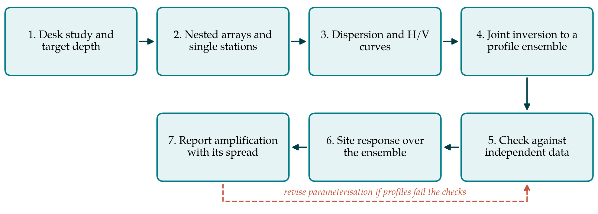
The workflow has seven steps, shown in Figure 1. The return path in the figure reflects the fact that the inversion is conditional on choices made by the analyst, and that those choices should be revisited when the result conflicts with independent knowledge of the site.

Figure 1: Proposed workflow from desk study to reporting of site amplification for a deep basin site

3.1. Step 1: Desk study and target depth

The geological setting decides the design of the survey. Geological maps, water-well and exploration logs, gravity or seismic reflection data and any earlier geophysical work are collected to estimate the likely depth to stiff rock and the nature of the main interfaces. The longest wavelength that must be measured follows from this depth, on the common rule of thumb that surface waves resolve structure to between one third and one half of their wavelength (Foti et al., 2018). The desk study should also flag evidence of strong lateral variation, such as proximity to the basin edge, since this bears on whether a one-dimensional interpretation is defensible.

3.2. Step 2: Acquisition

A single array cannot cover the full range of wavelengths. The proposal is to deploy nested arrays of increasing aperture around a common centre, each recorded for long enough to obtain stable averages at its lowest frequency of interest, with the largest aperture comparable to the target depth. Sensors must have adequate response at the lowest frequency sought; for deep basins this generally means broadband or intermediate-period seismometers, since ordinary geophones lose sensitivity below a few hertz. Sensor positions are surveyed and the instruments are recorded together beforehand to check their relative response. Single-station recordings for spectral ratios are taken at the array centre and at several points across the footprint, and a short active survey at the centre supplies the high-frequency end of the dispersion curve.

3.3. Step 3: Dispersion and spectral ratio curves

Each array is processed by both frequency-wavenumber and spatial autocorrelation methods. Phase velocity estimates are retained only within the wavenumber limits of the array, which are obtained from its theoretical response, and the segments from the different apertures are merged into one curve with an uncertainty at each frequency derived from the scatter between time windows. Where the techniques disagree beyond that scatter the cause is sought before proceeding: an uneven source distribution, a higher mode mistaken for the fundamental, or lateral variation beneath the array. Spectral ratios are computed following the SESAME recommendations, and the peak frequency is accepted only if it meets their reliability criteria and is consistent across the footprint.

3.4. Step 4: Joint inversion

The dispersion curve and the spectral ratio peak frequency, or the ellipticity curve where it can be extracted with confidence, are inverted together with a direct-search algorithm (Wathelet et al., 2004). The parameterisation is the most consequential choice. Several layering schemes of differing complexity are run, each informed by the desk study, and no scheme is preferred merely because it attains the lowest misfit. From the models that fit the data within their uncertainty, a manageable set of profiles is drawn for the later analysis. Compression wave velocity and density are weakly resolved and are tied to shear wave velocity through plausible ranges of Poisson's ratio, with allowance for saturation below the water table.

3.5. Step 5: Checks against independent data

Before the profiles are used they are compared with whatever was not used to derive them: borehole logs that fix the depth of a stratigraphic boundary, any downhole velocity measurements in the upper part of the column, and the theoretical resonance frequency of each profile set against the observed spectral ratio peaks at other points on the site. The InterPACIFIC comparisons found that surface wave and invasive methods agree well on average velocity and less well on the depth and sharpness of individual interfaces (Garofalo et al., 2016), so the checks should concentrate on interfaces. Profiles that contradict firm independent evidence are discarded, and if most of them do, the parameterisation is revised and the inversion repeated.

3.6. Step 6: Site response analysis over the ensemble

Each retained profile is analysed for vertically propagating shear waves, by the equivalent-linear method in the tradition of SHAKE (Schnabel et al., 1972) or by a nonlinear time-domain code where the expected strains warrant it. Modulus reduction and damping curves are assigned by soil type and confining pressure, for which the relations of Darendeli (2001) are widely used, although their extrapolation to the pressures found at depth in a thick basin is itself uncertain. Input motions are defined at the reference horizon identified by the inversion and selected to be consistent with the hazard at that horizon, in the manner recommended by Stewart et al. (2014). Small-strain damping deserves attention in deep profiles, because its effect accumulates over a long travel path.

3.7. Step 7: Reporting

The product is a set of amplification functions and surface spectra, one for each profile and motion, summarised by a central estimate and a measure of spread. The report should separate the contribution of the velocity model from that of the input motions and the nonlinear properties, and should state the frequency range over which the dispersion data constrain the profile. Below the lowest resolved frequency the result rests on the spectral ratio peak and on geological inference, and the reader needs to be told so.

4. Fitting the Workflow to Practice

The effort involved is dominated by fieldwork. Large-aperture arrays need access to land over several hundred metres in every direction, which in an urban basin usually means parks, car parks and road verges and an irregular geometry; the modified autocorrelation method tolerates this. Recording at night reduces transient disturbance close to sensors without removing the low-frequency energy that matters for depth. Processing and inversion can be done entirely with open-source tools. Where the budget allows a single deep borehole, placing it at the array centre gives the most value, because it anchors the interfaces that surface waves resolve least well and provides samples for laboratory measurement of nonlinear properties.

5. Limitations and What Remains to Be Shown

The workflow yields a one-dimensional description of a three-dimensional structure. Sediment-filled valleys trap and focus energy, generate surface waves at their edges and can resonate as a whole, with amplification and duration that horizontally layered models underestimate (Bard and Bouchon, 1985). The procedure does not capture these effects, and where the desk study or the spatial pattern of spectral ratios points to them, two- or three-dimensional modelling or empirical correction is needed in addition.

Since the procedure has not been tested here, its performance is a matter for future work. A convincing validation would apply it at basin sites that have both a deep velocity log and recordings of earthquakes at the surface and at depth, and would ask two things: whether the measured profile falls inside the ensemble, and whether the spread of computed amplification encloses the observed amplification over the resolved frequency band. It would also show how the outcome changes with the number of profiles drawn and with the layering schemes tried, which at present are left to the analyst's judgement.

6. Conclusion

Ambient vibration arrays offer a practical means of extending velocity profiles to the depths that govern the response of thick alluvial deposits. The workflow proposed here joins established techniques in a fixed order, uses two array methods and the spectral ratio to constrain each other, and carries an ensemble of profiles through to the amplification estimate so that the limits of the data remain visible to those who use the result. It is offered as a starting point for application and testing at well-characterised sites.

Conflict of interest

To be declared by the author(s) before publication.

Funding

To be declared by the author(s) before publication.

References

[1] Aki, K. Space and time spectra of stationary stochastic waves, with special reference to microtremors. Bulletin of the Earthquake Research Institute, University of Tokyo 35, 415-456 (1957).
[2] Bard, P.-Y. and Bouchon, M. The two-dimensional resonance of sediment-filled valleys. Bulletin of the Seismological Society of America 75(2), 519-541 (1985).
[3] Bettig, B., Bard, P.-Y., Scherbaum, F., Riepl, J., Cotton, F., Cornou, C. and Hatzfeld, D. Analysis of dense array noise measurements using the modified spatial auto-correlation method (SPAC): Application to the Grenoble area. Bollettino di Geofisica Teorica ed Applicata 42(3-4), 281-304 (2001).
[4] Bonnefoy-Claudet, S., Cotton, F. and Bard, P.-Y. The nature of noise wavefield and its applications for site effects studies: A literature review. Earth-Science Reviews https://doi.org/10.1016/j.earscirev.2006.07.004 79(3-4), 205-227 (2006).
[5] Capon, J. High-resolution frequency-wavenumber spectrum analysis. Proceedings of the IEEE https://doi.org/10.1109/PROC.1969.7278 57(8), 1408-1418 (1969).
[6] Darendeli, M.B. Development of a new family of normalized modulus reduction and material damping curves. PhD dissertation, University of Texas at Austin (2001).
[7] Foti, S., Hollender, F., Garofalo, F., Albarello, D., Asten, M., Bard, P.-Y., Comina, C., Cornou, C., Cox, B., Di Giulio, G., Forbriger, T., Hayashi, K., Lunedei, E., Martin, A., Mercerat, D., Ohrnberger, M., Poggi, V., Renalier, F., et al. Guidelines for the good practice of surface wave analysis: A product of the InterPACIFIC project. Bulletin of Earthquake Engineering https://doi.org/10.1007/s10518-017-0206-7 16(6), 2367-2420 (2018).
[8] Garofalo, F., Foti, S., Hollender, F., Bard, P.-Y., Cornou, C., Cox, B.R., Dechamp, A., Ohrnberger, M., Perron, V., Sicilia, D., Teague, D. and Vergniault, C. InterPACIFIC project: Comparison of invasive and non-invasive methods for seismic site characterization. Part II: Inter-comparison between surface-wave and borehole methods. Soil Dynamics and Earthquake Engineering 82, 241-254 (2016).
[9] Nakamura, Y. A method for dynamic characteristics estimation of subsurface using microtremor on the ground surface. Quarterly Report of the Railway Technical Research Institute 30(1), 25-33 (1989).
[10] Park, C.B., Miller, R.D. and Xia, J. Multichannel analysis of surface waves. Geophysics https://doi.org/10.1190/1.1444590 64(3), 800-808 (1999).
[11] Sambridge, M. Geophysical inversion with a neighbourhood algorithm - I. Searching a parameter space. Geophysical Journal International 138(2), 479-494 (1999).
[12] Scherbaum, F., Hinzen, K.-G. and Ohrnberger, M. Determination of shallow shear wave velocity profiles in the Cologne, Germany area using ambient vibrations. Geophysical Journal International 152(3), 597-612 (2003).
[13] Schnabel, P.B., Lysmer, J. and Seed, H.B. SHAKE: A computer program for earthquake response analysis of horizontally layered sites. Report EERC 72-12, Earthquake Engineering Research Center, University of California, Berkeley (1972).
[14] SESAME Guidelines for the implementation of the H/V spectral ratio technique on ambient vibrations: Measurements, processing and interpretation. SESAME European Research Project, WP12, Deliverable D23.12 (2004).
[15] Stewart, J.P., Afshari, K. and Hashash, Y.M.A. Guidelines for performing hazard-consistent one-dimensional ground response analysis for ground motion prediction. PEER Report 2014/16, Pacific Earthquake Engineering Research Center, Berkeley, CA (2014).
[16] Teague, D.P. and Cox, B.R. Site response implications associated with using non-unique Vs profiles from surface wave inversion in comparison with other commonly used methods of accounting for Vs uncertainty. Soil Dynamics and Earthquake Engineering 91, 87-103 (2016).
[17] Wathelet, M., Chatelain, J.-L., Cornou, C., Di Giulio, G., Guillier, B., Ohrnberger, M. and Savvaidis, A. Geopsy: A user-friendly open-source tool set for ambient vibration processing. Seismological Research Letters 91(3), 1878-1889 (2020).
[18] Wathelet, M., Jongmans, D. and Ohrnberger, M. Surface-wave inversion using a direct search algorithm and its application to ambient vibration measurements. Near Surface Geophysics 2(4), 211-221 (2004).

Article metrics

0 total accesses since publication. 0 citing articles have been indexed to date.