1. Introduction
Muons produced by cosmic ray interactions in the upper atmosphere are the most numerous charged particles at sea level. The integral intensity there is close to one particle per square centimetre per minute through a horizontal surface, and the standard reference data are collected in the review of the Particle Data Group (Workman et al., 2022) and in the compilation of Grieder (2001). The flux rises with altitude, and following that rise has been a classic exercise since the early days of the subject (Rossi, 1948).
The instruments available for the exercise have changed. A slab of plastic scintillator coupled to a silicon photomultiplier and read by a microcontroller can be built for a small fraction of the cost of a photomultiplier tube system, runs from a battery and weighs little. Published open designs, of which the desktop detector of Axani et al. (2017) and its successor (Axani et al., 2018) are the best known, have put arrays of such counters into many hands. They are attractive for work at mountain stations and on balloons, where mass and power are limited.
Low cost does not remove the need for calibration; it increases it, because inexpensive counters differ from one another and drift with temperature. This article proposes a procedure by which a small group can convert coincidence rates from such an array into a muon flux with a stated uncertainty. It is a method paper. No measurements are reported, and the procedure has not been tested here against an independent instrument.
2. Background
Two matters need to be understood before the steps make sense: what a scintillator telescope actually counts at altitude, and where inexpensive hardware departs from the ideal counter of the textbooks.
2.1. What a scintillator telescope counts
A relativistic muon crossing plastic scintillator deposits roughly two megaelectronvolts per centimetre of path, and a counter registers it when the resulting light pulse exceeds a threshold. Any charged particle does the same. At sea level the particles that pass through two separated counters in coincidence are mostly muons, with electrons and positrons as the main contamination. Higher up the proportions change: the electromagnetic component and the surviving protons grow faster than the muons (Gaisser et al., 2016). The historical remedy was to define a hard component as the part of the radiation able to penetrate ten or more centimetres of lead (Rossi, 1948). A telescope without absorber measures the total charged flux, and a claim to have measured muons at altitude must say how the other particles were removed or estimated.
The muon flux also depends on direction, falling off from the vertical approximately as the square of the cosine of the zenith angle at sea level, on the geomagnetic cutoff rigidity of the site (Smart and Shea, 2005), and on the state of the atmosphere. Higher surface pressure means more absorbing mass overhead and a lower rate. Temperature in the upper atmosphere alters the height at which muons are produced and so the fraction that decay in flight, an effect first explained by Blackett (1938) and treated at length by Dorman (2004).
2.2. Where low-cost counters depart from the ideal
A silicon photomultiplier is an array of avalanche photodiodes operated a few volts above breakdown. Its gain is proportional to that excess voltage, and the breakdown voltage itself rises with temperature, so that at fixed bias the gain falls as the device warms. Thermally generated dark counts, optical crosstalk between cells and afterpulsing add pulses that have nothing to do with particles (Renker and Lorenz, 2009). A mountain hut or a balloon gondola may span tens of degrees in a day. Small scintillator tiles collect light unevenly, and hand-made optical couplings vary from one counter to the next. Microcontroller readout has a dead time of some microseconds to milliseconds per event that is rarely documented. None of this prevents a good measurement, but each item must be measured and not assumed.
3. The Proposed Procedure
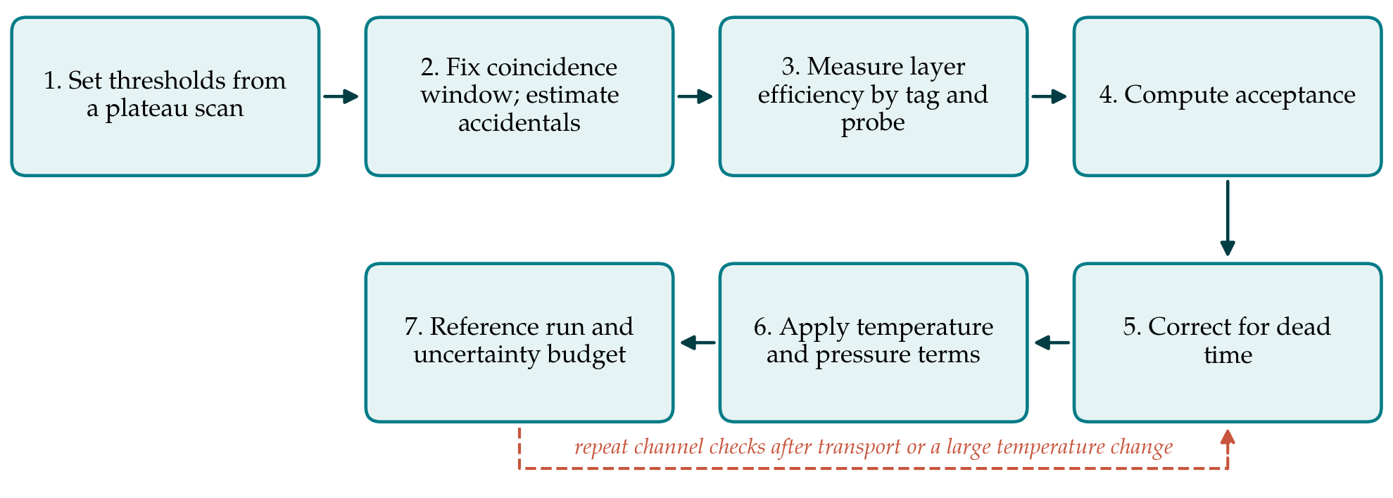
The procedure assumes an array of at least three counters that can be stacked as a telescope, a temperature sensor in contact with the photosensors, a barometer, and a readout that records a time stamp and a pulse height for each channel. Table 1 lists the seven steps with the quantity each determines, and Figure 1 shows their order. The principles are those of standard texts on detectors (Knoll, 2010; Leo, 1994).
| Step | Quantity determined | Accompanying check |
|---|---|---|
| 1. Threshold plateau scan | Operating threshold for each channel | Coincidence rate flat over a range of thresholds |
| 2. Coincidence window | Resolving time and accidental rate | Delayed-coincidence rate agrees with the calculated value |
| 3. Tag and probe | Efficiency of each layer | Repeat with layers permuted |
| 4. Acceptance | Geometric factor of the telescope | Analytic value against Monte Carlo |
| 5. Dead time | Live fraction of each run | Rate from a pulser recovered correctly |
| 6. Environment | Temperature and pressure coefficients | Residual rate uncorrelated with either |
| 7. Reference run | Overall normalisation and uncertainty budget | Sea-level result consistent with published intensity |
3.1. Step 1: Set thresholds from a plateau scan
With two counters in coincidence, the threshold of one is varied while the other is held fixed, and the coincidence rate is recorded at each setting. At low thresholds the rate is inflated by noise; at high thresholds real particles are lost. Between them there should be a plateau on which the rate changes little, and the operating point is set near its lower third. A counter that shows no plateau has too little light and should be rebuilt before it is used. The scan is repeated for every channel and again at the highest and lowest temperatures expected in the field.
3.2. Step 2: Fix the coincidence window and estimate accidentals
The distribution of time differences between channels gives the resolving time. For two channels with singles rates R1 and R2 and a resolving time τ, the expected accidental rate is 2τR1R2. The calculation is checked by inserting a delay much longer than the window in one channel, so that only chance coincidences remain. Because singles rates in silicon photomultiplier counters are dominated by dark counts and rise with temperature, the accidental rate is recomputed for every run from the singles recorded in that run.
3.3. Step 3: Measure layer efficiency by tag and probe
Three counters are stacked with the one under test in the middle. A coincidence of the outer pair tags a particle that must have crossed the middle counter, provided the outer pair is no larger than the middle one. The efficiency of the middle counter is the ratio of threefold to twofold coincidences, after accidentals are subtracted from both. The counters are then permuted so that each takes the middle position in turn. The efficiency is recorded as a function of temperature, since a falling gain moves pulses toward the threshold.
3.4. Step 4: Compute the acceptance
The rate of a telescope equals the directional intensity integrated over its area and solid angle. For simple geometries the geometric factor can be written in closed form, and the expressions of Sullivan (1971) cover rectangular and circular coaxial elements for isotropic and cosine-power angular distributions. The analytic value is checked with a short Monte Carlo calculation that throws tracks through the measured geometry. A full simulation of the secondary flux and the detector response, for instance with the CRY generator (Hagmann et al., 2007) or CORSIKA (Heck et al., 1998) feeding Geant4 (Agostinelli et al., 2003), is not required for the acceptance but is needed for the particle composition discussed below.
3.5. Step 5: Correct for dead time
The dead time per event is measured by driving the readout with a pulse generator at known rates and finding the rate at which recorded counts begin to fall short. For a non-paralysable system with dead time τd and recorded rate m, the true rate is m/(1 - mτd) (Knoll, 2010). Where the firmware permits, a live-time counter is preferable to a formula. The correction is small at sea level and can become appreciable at balloon altitudes, where rates are many times higher.
3.6. Step 6: Apply temperature and pressure terms
Two environmental effects must be kept apart. One is instrumental: the dependence of efficiency on photosensor temperature, already measured in step 3, or removed at source by adjusting the bias voltage with temperature to hold the gain constant. The other is atmospheric: the dependence of the true flux on pressure. The barometric coefficient for muons is of the order of a tenth of a percent per hectopascal and negative, and it is found by regressing the efficiency-corrected rate on pressure over a period of stable operation at one site. Data from a nearby neutron monitor, whose response to primary variations is well characterised (Simpson, 2000), help to separate changes in the primary flux from changes in the atmosphere.
3.7. Step 7: Make a reference run and close the uncertainty budget
Before the array is taken to altitude it is run for several days at a low-altitude site, and the corrected flux is compared with the published sea-level intensity for that latitude (Workman et al., 2022). Agreement within the combined uncertainty supports the chain of corrections; disagreement must be traced before the campaign proceeds. The uncertainty budget is then written out following the international guide (JCGM, 2008), with statistical terms from Poisson counting and separate systematic terms for efficiency, acceptance, accidentals, dead time and environmental coefficients.
4. Fitting the Procedure to High-Altitude Conditions
At a mountain site the procedure applies almost unchanged, with two additions. Steps 1 to 3 are repeated on arrival, because transport disturbs optical couplings and the temperature regime is new. And the composition problem must be faced. The straightforward approach is to place lead between the lower counters and to report the hard component so defined, stating the absorber thickness. Where the mass of lead is prohibitive, the alternative is to report the total charged-particle flux and to estimate the muon fraction from simulation at the site's altitude and cutoff, with the dependence on the model carried as a systematic uncertainty.
On a balloon the conditions are harsher. Temperature falls far below the range of a bench test and then recovers, pressure drops by two orders of magnitude, and the gondola rotates and swings. Efficiency should be monitored in flight by keeping a threefold arrangement active throughout, so that step 3 runs continuously. Lead is seldom carried, and near the altitude of maximum ionisation the muon is a minority particle; the result of such a flight is better described as a charged-particle profile.
5. Limitations and What Remains to Be Shown
The procedure is proposed and untested. Its central claim, that seven steps within the means of a small group yield a flux with a defensible uncertainty, would be established by operating a calibrated low-cost array beside a reference telescope of known response at two or more altitudes and comparing the results. Such a comparison would also show which term dominates the budget in practice. It is plausible that the efficiency and its temperature dependence dominate at mountain sites and that particle composition dominates at balloon altitudes, but this is an expectation and not a result.
Several effects are left out. Tag-and-probe efficiency is an average over the area of the outer counters and hides non-uniform light collection near the edges of a tile. Showers that strike several counters at once are treated as single particles. The angular distribution is assumed and not measured, and its form changes with altitude. A group needing accuracy better than a few percent would have to address each of these.
6. Conclusion
Inexpensive scintillator counters can support quantitative cosmic ray measurements at altitude if the path from count rate to flux is calibrated step by step. The procedure proposed here orders the necessary measurements so that each depends only on those before it, pairs every determination with a check, and ends with a reference run that tests the whole chain against a known value. Its adequacy is for comparison measurements to decide. In the meantime it offers groups using these instruments a common and explicit basis on which results from different arrays and sites can be compared.
Conflict of interest
To be declared by the author(s) before publication.
Funding
To be declared by the author(s) before publication.