1. Introduction
Radio spectrum is finite, and two transmitters that are close together cannot use the same channel without degrading each other's signal. If transmitters are drawn as vertices and each interfering pair as an edge, a conflict-free plan is a proper colouring of the resulting graph, and the smallest number of channels that suffices is its chromatic number. The observation is simple, but it tied a practical engineering task to a problem that mathematicians had studied since the four colour conjecture, and the exchange between the two has run in both directions ever since.
The link was made systematic by Hale (1980), who classified frequency assignment problems by their constraints and objectives and showed that each could be stated as a generalised colouring problem. The generalisations were needed because real interference is not only co-channel. Adjacent channels leak into one another, transmitters on the same mast need wide separations, and what is minimised is often the width of the band occupied and not the number of channels used. Each of these features produced a new colouring parameter, and for each the first questions were the same: how small can it be, how large can it be, and how hard is it to compute.
This article reviews the answers. It concentrates on bounds, because bounds are what a planner can use before any optimisation is run: a lower bound says how much spectrum must be requested, and an upper bound with a constructive proof supplies an assignment. Later sections cover the classical chromatic number, T-colourings and distance labellings, special graph classes that model real networks, and complexity and algorithms.
2. Scope and Approach
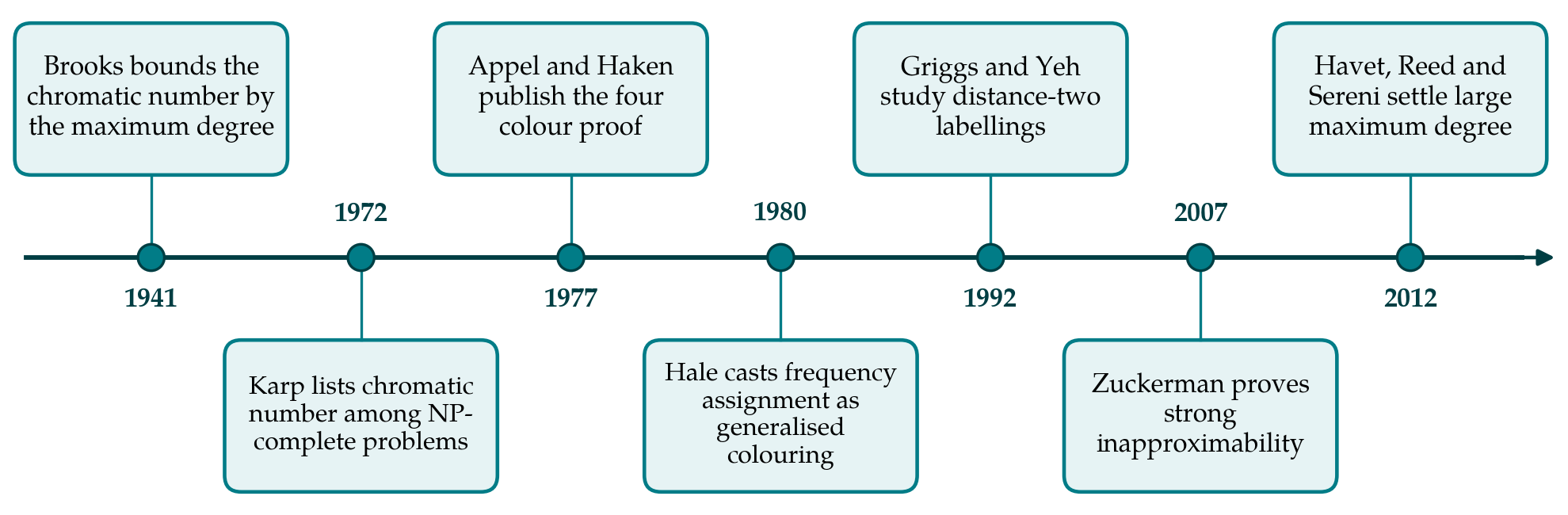
The review is a narrative account of the published literature, organised by type of bound. It draws on the standard references in graph colouring (Jensen and Toft, 1995), on the surveys of frequency assignment by Murphey et al. (1999) and Aardal et al. (2007), on the survey of distance labellings by Calamoneri (2011), and on the original papers in which the main bounds were proved. It does not attempt an exhaustive bibliography, and it leaves aside dynamic and online channel allocation, where the questions are of a different kind. Throughout, G is a finite simple graph with n vertices, maximum degree Δ, clique number ω and chromatic number χ. Figure 1 marks the results around which the account is organised.
3. Bounds on the Chromatic Number
Table 1 collects the bounds discussed in this section and the next, with a note on how each is read in a frequency assignment setting.
| Bound | Statement | Reading for frequency assignment | Source |
|---|---|---|---|
| Clique | χ is at least ω | A set of mutually interfering transmitters needs distinct channels | Jensen and Toft, 1995 |
| Hoffman | χ is at least 1 − λ /λ max min | Lower bound computable from the adjacency spectrum | Hoffman, 1970 |
| Theta function | ω ≤ ϑ of the complement ≤ χ | Polynomial-time lower bound, at least as strong as the clique bound | Lovász, 1979 |
| Brooks | χ ≤ Δ unless G is complete or an odd cycle | Channels needed never exceed the largest number of interferers, with two exceptions | Brooks, 1941 |
| Welsh-Powell | χ ≤ max over i of min(d + 1, i i) | Guarantee for greedy assignment in order of decreasing degree | Welsh and Powell, 1967 |
| Wilf | χ ≤ 1 + λ max | Upper bound that reflects average and not only worst-case density | Wilf, 1967 |
| Griggs-Yeh | 2 λ ≤ Δ + 2Δ; conjectured ≤ 2,1 2 Δ | Span sufficient when adjacent channels are also constrained | Griggs and Yeh, 1992 |
3.1. Lower bounds
The elementary lower bound is the clique number: vertices that are pairwise adjacent need pairwise different colours. A second elementary bound comes from independence, since every colour class is an independent set and so χ is at least n divided by the independence number. In interference graphs derived from geography the clique bound is usually the informative one, because transmitters cluster in cities and around shared sites. It can nevertheless be arbitrarily weak in principle. Erdős (1959) proved by a probabilistic argument that there are graphs with no short cycles, and hence no triangles, whose chromatic number is as large as desired, so no function of ω bounds χ from above on general graphs.
Spectral methods give lower bounds of a different character. Hoffman (1970) showed that χ is at least 1 − λmax/λmin, where λmax and λmin are the largest and smallest eigenvalues of the adjacency matrix. The theta function of Lovász (1979), introduced to determine the Shannon capacity of the pentagon, refines this: its value on the complement of G lies between ω and χ and can be computed to any accuracy in polynomial time by semidefinite programming. The sandwich property is notable because both ω and χ are hard to compute. For perfect graphs, where ω and χ agree on every induced subgraph, it yields a polynomial algorithm for the chromatic number. Interval graphs, which model transmitters along a line such as a road or a river valley, are perfect, and for them the clique bound is exact.
3.2. Upper bounds
Colouring the vertices one at a time, giving each the smallest colour not used on its neighbours, needs at most Δ + 1 colours. Brooks (1941) proved that Δ colours suffice for a connected graph unless it is a complete graph or an odd cycle. The greedy argument is sensitive to the order of the vertices, and better orders give better bounds. Welsh and Powell (1967) showed that colouring in order of decreasing degree uses at most the maximum over i of min(di + 1, i) colours, where di is the i-th largest degree. Ordering so that each vertex has few earlier neighbours leads to the degeneracy bound: if every subgraph has a vertex of degree at most k, then χ ≤ k + 1. The spectral counterpart is the bound χ ≤ 1 + λmax of Wilf (1967). It is never worse than Δ + 1 and never better than the degeneracy bound, because λmax is at most Δ and at least the minimum degree of every subgraph.
For frequency planning the constructive nature of these proofs matters as much as the numbers. Each is an algorithm, and each explains a rule of thumb used by engineers: assign the most constrained transmitters first. The DSATUR heuristic of Brélaz (1979), which always colours next the vertex that sees the most distinct colours among its neighbours, is the dynamic form of the same idea and remains a standard starting point.
4. Generalised Colourings Motivated by Frequency Assignment
Proper colouring models co-channel interference only. Two generalisations capture the further constraints that arise in practice.
4.1. T-colourings
In the formulation of Hale (1980), channels are positive integers and a set T of nonnegative integers containing zero lists the separations forbidden between interfering transmitters. A T-colouring assigns to each vertex an integer so that the labels of adjacent vertices never differ by an element of T. Two objectives compete. The order is the number of distinct labels used; the span is the difference between the largest and the smallest. The minimum order always equals χ, so nothing new arises there, but the minimum span depends on T in subtle ways. Cozzens and Roberts (1982) proved that the T-span of G lies between the T-spans of the complete graphs on ω and on χ vertices, which reduces the problem to complete graphs whenever ω = χ. When T consists of the integers from 0 to r, the span is exactly (r + 1)(χ − 1). For other sets even the complete graph case is unresolved, and Roberts (1991) surveyed what was known and what was open. A further complication is that an assignment of minimum span need not use the minimum number of channels, so the two objectives cannot always be met together.
4.2. Distance-constrained labellings
A different refinement asks that transmitters which are very close differ by at least two channels and those which are merely close differ by at least one. In graph terms an L(2,1)-labelling assigns nonnegative integers so that adjacent vertices differ by at least two and vertices at distance two receive different labels; the smallest achievable maximum label is written λ2,1. Griggs and Yeh (1992), who credit the problem to Roberts, showed that determining λ2,1 is NP-complete, that it is at least Δ + 1, that for trees it is either Δ + 1 or Δ + 2, and that in general it is at most Δ2 + 2Δ. They conjectured that Δ2 is the right upper bound when Δ is at least two.
The conjecture has guided the subject. Chang and Kuo (1996) improved the bound to Δ2 + Δ by a labelling algorithm that also gives exact values on several graph classes, Gonçalves (2008) reduced it to Δ2 + Δ − 2, and Havet et al. (2012) proved the conjecture for all sufficiently large Δ. For small maximum degree it remains open. The quadratic order of the bound cannot be improved, since in a graph of diameter two all labels must be distinct and such graphs can have close to Δ2 vertices. The survey of Calamoneri (2011) records the known values for the general L(h, k) problem class by class.
5. Structured Interference Graphs
General bounds are pessimistic for graphs that come from geometry. If the interference graph is planar, four channels suffice, by the theorem of Appel and Haken (1977). Planarity is a reasonable model only when each transmitter interferes with its immediate neighbours, and a more flexible model is the unit disk graph, in which transmitters are points in the plane and two are adjacent when their distance is below a threshold. Clark et al. (1990) showed that colouring unit disk graphs is NP-hard although a maximum clique can be found in polynomial time, and Gräf et al. (1998) gave algorithms that use at most three times the optimal number of colours. The chromatic number of a unit disk graph is therefore within a constant factor of its clique number, in sharp contrast with the general case.
Cellular networks add demand. Base stations sit on the triangular lattice, each cell requires a given number of channels, and channels may be reused only in cells that are not adjacent. The task is a weighted colouring of an induced subgraph of the lattice. McDiarmid and Reed (2000) proved that this problem is NP-hard and gave a polynomial algorithm whose output is within a factor of about four thirds of the weighted clique bound. The result explains why reuse patterns based on small clusters of cells perform well: on the lattice the local clique bound is never far from the truth.
6. Complexity and Algorithms
Deciding whether a graph can be coloured with a given number of colours was on the original list of NP-complete problems of Karp (1972), and it is known to stay NP-complete for three colours on planar graphs of small maximum degree. Approximation is no easier. Zuckerman (2007) showed that, unless P equals NP, no polynomial algorithm approximates the chromatic number of an n-vertex graph within a factor of n raised to any fixed power below one. Every frequency assignment model that contains graph colouring inherits these limits, which is why bounds for restricted classes carry so much weight.
Practice relies on heuristics checked against lower bounds. Sequential methods of greedy and DSATUR type are fast and are used to initialise local search. The tabu search of Hertz and de Werra (1987) set the pattern for much of what followed. The survey of Aardal et al. (2007) compares these methods with integer programming and constraint satisfaction on public benchmark sets, and describes the lower bounding techniques that certify quality: clique bounds, bounds from travelling salesman relaxations on subsets of mutually constrained transmitters, and polyhedral bounds. Murphey et al. (1999) give a parallel account with more emphasis on the optimisation models.
7. Gaps and Directions for Further Work
The mathematical agenda is clear in outline. The conjecture of Griggs and Yeh is open for small maximum degree. T-spans of complete graphs are unknown for most forbidden sets. For unit disk graphs the best constant relating χ to ω has not been determined, and little is known when transmission ranges differ, which destroys the unit disk structure.
The modelling agenda is less tidy. A graph records interference as a relation between pairs, whereas a receiver is affected by the sum of all unwanted signals. A plan that satisfies every pairwise constraint can still fail when many weak interferers add up, and a plan that violates a constraint slightly may be acceptable. Formulations that minimise total interference address this, but the colouring bounds reviewed here then apply only to relaxations, and their tightness in that role has not been studied systematically (Aardal et al., 2007). Newer spectrum regimes, in which channels have unequal widths and may be aggregated, raise colouring problems that the classical parameters do not cover.
8. Conclusion
Graph colouring gives frequency planning a language and a set of guarantees. Clique and spectral lower bounds say how much spectrum is unavoidable, greedy and degree-based upper bounds come with assignments attached, and the generalisations to forbidden separations and distance constraints extend both kinds of statement to more realistic interference. On general graphs the guarantees are weak and provably cannot be much improved by efficient algorithms. On the graph classes that describe real networks they are strong, often within a small constant factor of optimal. The remaining distance between theory and practice lies mainly in what the graph leaves out, and narrowing it is as much a matter of modelling as of proving sharper bounds.
Conflict of interest
To be declared by the author(s) before publication.
Funding
To be declared by the author(s) before publication.