International Journal of Embedded Systems and Design

Tiny Machine Learning on Microcontrollers: Model Compression Techniques and Deployment Toolchains

Siddharth Figueroa¹, Dawit Jimenez², Lilit Choi³

¹ Department of Electrical Electronics, Anatolian Graduate Institute of Electrical Electronics, France, ² Department of Electrical Electronics, Chao Phraya University Centre for Electrical Electronics, Nepal, ³ Department of Electrical Electronics, Anatolian Research Institute of Electrical Electronics, Bahrain

Published 06 May 2026 Vol. 1, Article 2 10.62715/ijesd.2026.v1.i1.pp8-13 0 accesses 0 citations

Download PDF XML HTML EPUB

0Accesses

0Citations

Abstract

Running neural networks on microcontrollers, a practice now widely called tiny machine learning, places inference on devices with kilobytes of memory, no operating system and a power budget measured in milliwatts or less. This narrative review surveys the two bodies of work that make such deployment possible. The first is model compression: efficient architectures built from depthwise separable convolutions, pruning of weights and filters, quantisation to low-precision integers, knowledge distillation, and neural architecture search constrained by memory. The second is the deployment toolchain: interpreters such as TensorFlow Lite for Microcontrollers, optimised kernel libraries such as CMSIS-NN, compilers that turn a model into specialised code, and the benchmarks used to compare results. The review explains what each technique does, what it costs, and how the pieces fit together into a working pipeline. It identifies peak activation memory, more than parameter count, as the binding constraint on microcontrollers, and 8-bit post-training or quantisation-aware integer quantisation as the one technique that nearly every deployment uses. Gaps remain in the practical exploitation of unstructured sparsity, in on-device learning, in the portability of results across hardware, and in the verification of compressed models for applications where errors carry consequences.

Keywords: TinyML Microcontrollers Model compression Quantisation Pruning Embedded inference

1. Introduction

A typical microcontroller offers a single low-frequency core, a few hundred kilobytes of static memory at best, a megabyte or so of flash, and no memory management unit. Deep learning grew up on hardware many orders of magnitude larger. The work that closed part of this distance was reviewed for larger embedded processors by Sze et al. (2017), and the microcontroller case was brought to a wide engineering audience by Warden and Situnayake (2019), whose book also popularised the name TinyML.

The motivation is practical. Inference at the sensor avoids sending raw audio, images or vibration data over a radio, which saves energy and bandwidth and keeps the data on the device. It also lets a product respond without a network connection. Keyword spotting, the task of recognising a small spoken vocabulary, was the early demonstration that useful neural networks fit in this class of device (Zhang et al., 2017), and it remains a reference workload together with visual wake words, small image classification and anomaly detection.

Fitting a model into a microcontroller is a joint problem in machine learning and embedded software. The network must be made small, and the code that runs it must waste nothing. This review treats the two halves in turn, compression first and toolchains second, and then considers how they interact and what remains unsolved.

2. Scope and Approach

The article is a narrative review. It is built around the papers that introduced the main techniques and the tools that are in common use, as judged from their adoption in the field and in the community benchmark. It was not compiled through a systematic database search and does not attempt to list every proposal. Hardware accelerators and neuromorphic devices are outside its scope; the focus is the general-purpose 32-bit microcontroller, of which the Arm Cortex-M family is the usual example.

3. The Resource Constraints That Shape the Problem

Three budgets matter. Flash holds the weights and the code, so parameter count and numeric precision determine whether the model can be stored. Static memory holds the activations, the intermediate tensors passed between layers, and the requirement is set by the largest set of tensors that must be alive at once. Latency and energy follow from the number of arithmetic operations and from how well the kernels use the processor. Of the three, activation memory is usually the hardest. A convolutional network for images has its largest feature maps in the first layers, and a design that looks small by parameter count can still exceed the available memory many times over. Lin et al. (2020) make this point forcefully and design their system around the peak memory figure.

4. Model Compression Techniques

Compression methods are complementary and are normally combined. Table 1 summarises the main families, what each reduces and what it demands of the deployment software.

Table 1: Principal model compression techniques and their implications for microcontroller deployment
Technique	What it reduces	Requirement on the runtime	Representative source
Efficient architecture	Operations and parameters	Optimised depthwise and pointwise kernels	Howard et al., 2017
Unstructured pruning	Non-zero weights	Sparse storage and sparse kernels to realise any gain	Han et al., 2015
Structured pruning	Filters and channels	None; the result is a smaller dense network	Li et al., 2017
Integer quantisation	Bits per weight and activation	Integer-only kernels with fixed-point scaling	Jacob et al., 2018
Binarisation	Precision to one bit	Bitwise kernels; careful first and last layers	Courbariaux et al., 2016
Knowledge distillation	Accuracy lost by a small model	None; affects training only	Hinton et al., 2015
Constrained architecture search	Peak memory and latency	Accurate memory and latency model of the target	Lin et al., 2020

4.1. Efficient architectures

The cheapest operation is the one never performed, and the largest savings come from choosing a frugal architecture before any compression is applied. MobileNet replaced the standard convolution with a depthwise convolution followed by a pointwise one, cutting both operations and parameters, and exposed width and resolution multipliers that scale the network down smoothly (Howard et al., 2017). MobileNetV2 added inverted residual blocks with linear bottlenecks (Sandler et al., 2018). The depthwise separable networks that performed best in the keyword spotting study of Zhang et al. (2017) follow the same pattern, and most microcontroller vision and audio models today descend from these designs.

4.2. Pruning

Pruning removes parameters that contribute little. The idea predates deep learning: optimal brain damage used second-derivative information to select weights for deletion (LeCun et al., 1990). Han et al. (2015) showed that simple magnitude pruning followed by retraining removes a large share of the weights of modern networks with little loss of accuracy, and the lottery ticket hypothesis of Frankle and Carbin (2019) gave the observation a theoretical framing. On a microcontroller the distinction between unstructured and structured pruning is decisive. Unstructured pruning leaves a sparse matrix whose storage needs indices and whose multiplication needs irregular memory access, so the saving in flash is partial and the saving in time is often nil on a processor without sparse support. Structured pruning deletes whole filters or channels (Li et al., 2017) and yields a smaller dense network that any runtime executes faster. A critical survey by Blalock et al. (2020) also cautions that pruning results are hard to compare across papers because baselines and metrics differ.

4.3. Quantisation

Quantisation stores weights and activations at reduced precision. Moving from 32-bit floating point to 8-bit integers cuts model size by a factor of four and, as important, allows inference with integer arithmetic alone, which suits cores that lack a floating-point unit. The affine scheme of Jacob et al. (2018), in which a real value is represented by an integer, a scale and a zero point, is the basis of the formats used by the mainstream tools. Quantisation can be applied after training using a small calibration set, or simulated during training so that the network adapts to it; Krishnamoorthi (2018) sets out the practical trade-offs, and Gholami et al. (2021) survey the wider literature. Below eight bits, accuracy becomes harder to hold. Binarised networks constrain weights and activations to two values (Courbariaux et al., 2016) and replace multiplication with bitwise operations, at a cost in accuracy that has limited their use to simple tasks.

4.4. Distillation and combined pipelines

Knowledge distillation trains a small student network to reproduce the softened output distribution of a large teacher, which often recovers accuracy that the student would not reach from labels alone (Hinton et al., 2015). It changes nothing at deployment and combines freely with the other methods. Deep compression chained pruning, weight sharing and entropy coding into a single pipeline (Han et al., 2016) and established the habit of stacking techniques that TinyML work has followed since.

4.5. Architecture search under memory constraints

Manual design gives way to automated search once the constraint is stated precisely. SpArSe searched jointly over architecture and pruning for networks that fit microcontroller memory (Fedorov et al., 2019). MCUNet coupled a search over a space tailored to the memory limit with an inference engine tuned for the resulting models (Lin et al., 2020), and MicroNets used differentiable search with operation count as a proxy for latency on Cortex-M devices (Banbury et al., 2021a). The shared lesson is that the search must optimise the quantities the hardware imposes, peak memory above all, and not parameter count.

5. Deployment Toolchains

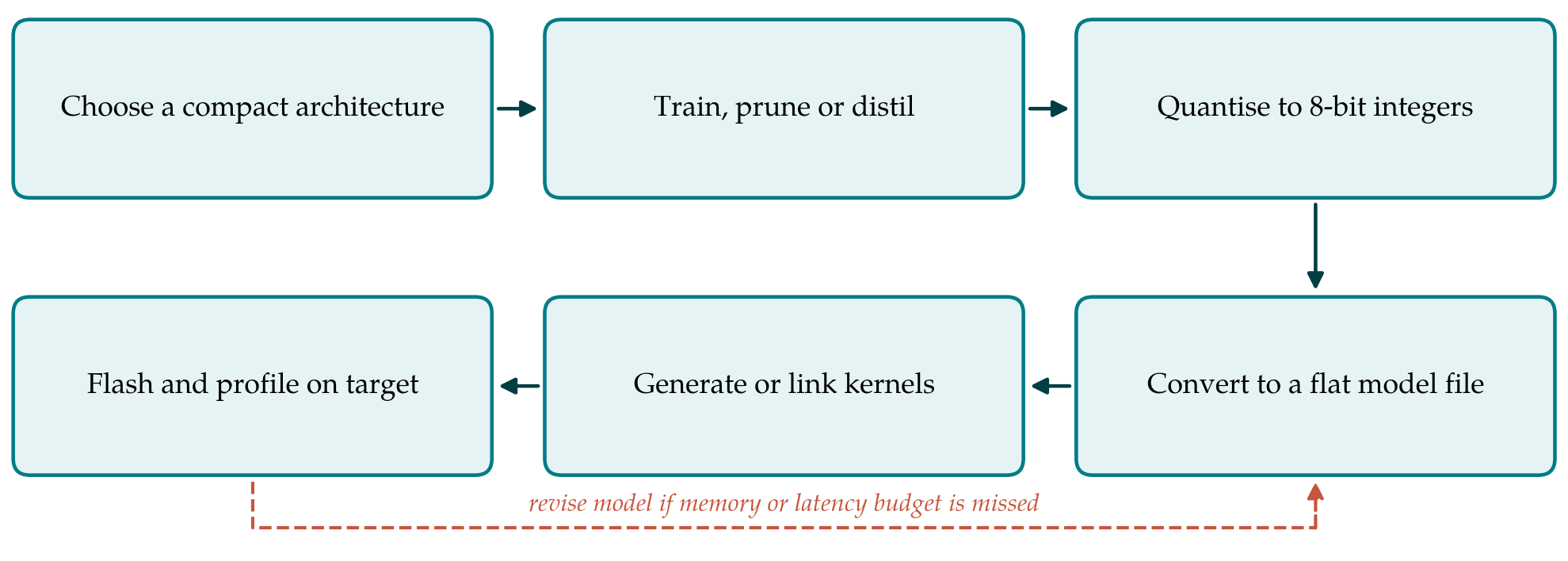
A trained and compressed model still has to become firmware. Figure 1 shows the usual sequence, from choice of architecture to profiling on the target, with the return path that is taken when the device budget is missed.

Figure 1: Typical pipeline from model design to profiled firmware on a microcontroller

5.1. Interpreters and kernel libraries

TensorFlow Lite for Microcontrollers is the most widely used runtime. It is an interpreter that reads a serialised model, plans tensor memory in a single arena supplied by the application, and dispatches each operator to a kernel. Its design avoids dynamic allocation and operating system dependencies so that it builds for bare-metal targets (David et al., 2021). Interpretation adds a small fixed overhead; most of the execution time is spent in the kernels. On Arm cores those kernels are commonly provided by CMSIS-NN, a library of fixed-point convolution, pooling and activation routines that use the processor's DSP extensions where present (Lai et al., 2018).

5.2. Compilers and code generators

The alternative to interpretation is compilation of the model into code specialised for it. TVM introduced a compiler stack with a tensor-level intermediate representation and automated tuning of operator implementations for a given target (Chen et al., 2018), and its microcontroller support emits C that links without a runtime interpreter. Silicon vendors provide generators of their own that take a quantised model and produce a C library for their parts. Code generation removes the interpreter and allows optimisations across layers, such as the in-place depthwise convolution used in MCUNet's engine. The price is a less transparent build and tighter coupling between model and firmware.

5.3. Benchmarks

Comparing results was difficult while every paper used its own model, dataset and board. The MLPerf Tiny suite defines four tasks, keyword spotting, visual wake words, image classification and anomaly detection, with reference models and rules for reporting latency, accuracy and energy (Banbury et al., 2021b). The keyword spotting task uses the Speech Commands dataset (Warden, 2018). The suite has given toolchain developers a common yardstick, though its workloads are small and do not cover every sensing application.

6. How Compression and Toolchain Interact

The two halves of the problem cannot be optimised separately. A compression method pays off only if the runtime has a kernel that exploits it: per-channel quantisation needs kernels that accept a scale for each output channel, a pruned filter saves time only when the converter removes it from the graph, and an operator the runtime does not implement stops deployment altogether. The memory planner matters as much as the kernels. Peak activation memory depends on the order in which operators are executed and on whether buffers are reused in place, so the same model file can fit under one runtime and overflow under another. For this reason careful projects measure on the target early, with a first model that is deliberately too simple, and treat the figures reported by the device as the specification that the next round of design must meet.

7. Gaps and Directions for Future Work

Four gaps stand out in the literature reviewed. Sparse models remain hard to exploit, since the mainstream runtimes execute dense kernels and unstructured sparsity gives little benefit without hardware or kernel support. Learning on the device is at an early stage: training needs gradients and stored activations that inference does not, and work on fitting it into microcontroller memory is recent. Portability is limited, because latency and memory depend on kernel implementations and memory planners that differ between runtimes and processor families, so a model tuned for one target may not fit another. Finally, the effect of compression on robustness is less studied than its effect on average accuracy. A quantised or pruned network can agree with its original on a test set and still differ on unusual inputs, which matters once such models are used in medical, industrial or automotive settings where behaviour must be argued and not only measured.

8. Conclusion

Machine learning on microcontrollers rests on a small set of well-understood ideas. Compact architectures built from depthwise separable convolutions set the starting point, integer quantisation is close to universal, structured pruning and distillation recover margin, and architecture search tuned to peak memory pushes furthest. On the software side an interpreter with optimised kernels serves most projects, with compilation available where every byte and cycle counts. The field's open questions lie less in making models smaller than in making the results portable, adaptable after deployment and trustworthy enough for applications in which a wrong answer has a cost.

Conflict of interest

To be declared by the author(s) before publication.

Funding

To be declared by the author(s) before publication.

References

[1] Banbury, C., Reddi, V.J., Torelli, P., Holleman, J., Jeffries, N., Kiraly, C., et al. MLPerf Tiny benchmark. Proceedings of the Neural Information Processing Systems Track on Datasets and Benchmarks (2021).
[2] Banbury, C., Zhou, C., Fedorov, I., Matas, R., Thakker, U., Gope, D., Janapa Reddi, V., Mattina, M. and Whatmough, P. MicroNets: Neural network architectures for deploying TinyML applications on commodity microcontrollers. Proceedings of Machine Learning and Systems 3 (2021).
[3] Blalock, D., Gonzalez Ortiz, J.J., Frankle, J. and Guttag, J. What is the state of neural network pruning?. Proceedings of Machine Learning and Systems 2, 129-146 (2020).
[4] Chen, T., Moreau, T., Jiang, Z., Zheng, L., Yan, E., Cowan, M., Shen, H., Wang, L., Hu, Y., Ceze, L., Guestrin, C. and Krishnamurthy, A. TVM: An automated end-to-end optimizing compiler for deep learning. Proceedings of the 13th USENIX Symposium on Operating Systems Design and Implementation (OSDI) 578-594 (2018).
[5] Courbariaux, M., Hubara, I., Soudry, D., El-Yaniv, R. and Bengio, Y. Binarized neural networks: Training deep neural networks with weights and activations constrained to +1 or -1. arXiv preprint arXiv:1602.02830 (2016).
[6] David, R., Duke, J., Jain, A., Janapa Reddi, V., Jeffries, N., Li, J., Kreeger, N., Nappier, I., Natraj, M., Regev, S., Rhodes, R., Wang, T. and Warden, P. TensorFlow Lite Micro: Embedded machine learning for TinyML systems. Proceedings of Machine Learning and Systems 3, 800-811 (2021).
[7] Fedorov, I., Adams, R.P., Mattina, M. and Whatmough, P.N. SpArSe: Sparse architecture search for CNNs on resource-constrained microcontrollers. Advances in Neural Information Processing Systems 32 (2019).
[8] Frankle, J. and Carbin, M. The lottery ticket hypothesis: Finding sparse, trainable neural networks. Proceedings of the 7th International Conference on Learning Representations (ICLR) (2019).
[9] Gholami, A., Kim, S., Dong, Z., Yao, Z., Mahoney, M.W. and Keutzer, K. A survey of quantization methods for efficient neural network inference. arXiv preprint arXiv:2103.13630 (2021).
[10] Han, S., Mao, H. and Dally, W.J. Deep compression: Compressing deep neural networks with pruning, trained quantization and Huffman coding. Proceedings of the 4th International Conference on Learning Representations (ICLR) (2016).
[11] Han, S., Pool, J., Tran, J. and Dally, W.J. Learning both weights and connections for efficient neural networks. Advances in Neural Information Processing Systems 28, 1135-1143 (2015).
[12] Hinton, G., Vinyals, O. and Dean, J. Distilling the knowledge in a neural network. arXiv preprint arXiv:1503.02531 (2015).
[13] Howard, A.G., Zhu, M., Chen, B., Kalenichenko, D., Wang, W., Weyand, T., Andreetto, M. and Adam, H. MobileNets: Efficient convolutional neural networks for mobile vision applications. arXiv preprint arXiv:1704.04861 (2017).
[14] Jacob, B., Kligys, S., Chen, B., Zhu, M., Tang, M., Howard, A., Adam, H. and Kalenichenko, D. Quantization and training of neural networks for efficient integer-arithmetic-only inference. Proceedings of the IEEE Conference on Computer Vision and Pattern Recognition (CVPR) https://doi.org/10.1109/CVPR.2018.00286 2704-2713 (2018).
[15] Krishnamoorthi, R. Quantizing deep convolutional networks for efficient inference: A whitepaper. arXiv preprint arXiv:1806.08342 (2018).
[16] Lai, L., Suda, N. and Chandra, V. CMSIS-NN: Efficient neural network kernels for Arm Cortex-M CPUs. arXiv preprint arXiv:1801.06601 (2018).
[17] LeCun, Y., Denker, J.S. and Solla, S.A. Optimal brain damage. Advances in Neural Information Processing Systems 2, 598-605 (1990).
[18] Li, H., Kadav, A., Durdanovic, I., Samet, H. and Graf, H.P. Pruning filters for efficient ConvNets. Proceedings of the 5th International Conference on Learning Representations (ICLR) (2017).
[19] Lin, J., Chen, W.-M., Lin, Y., Cohn, J., Gan, C. and Han, S. MCUNet: Tiny deep learning on IoT devices. Advances in Neural Information Processing Systems 33, 11711-11722 (2020).
[20] Sandler, M., Howard, A., Zhu, M., Zhmoginov, A. and Chen, L.-C. MobileNetV2: Inverted residuals and linear bottlenecks. Proceedings of the IEEE Conference on Computer Vision and Pattern Recognition (CVPR) https://doi.org/10.1109/CVPR.2018.00474 4510-4520 (2018).
[21] Sze, V., Chen, Y.-H., Yang, T.-J. and Emer, J.S. Efficient processing of deep neural networks: A tutorial and survey. Proceedings of the IEEE https://doi.org/10.1109/JPROC.2017.2761740 105(12), 2295-2329 (2017).
[22] Warden, P. Speech commands: A dataset for limited-vocabulary speech recognition. arXiv preprint arXiv:1804.03209 (2018).
[23] Warden, P. and Situnayake, D. TinyML: Machine Learning with TensorFlow Lite on Arduino and Ultra-Low-Power Microcontrollers. O'Reilly Media, Sebastopol, CA (2019).
[24] Zhang, Y., Suda, N., Lai, L. and Chandra, V. Hello edge: Keyword spotting on microcontrollers. arXiv preprint arXiv:1711.07128 (2017).

Article metrics

0 total accesses since publication. 0 citing articles have been indexed to date.