1. Introduction
The contents of a first course in numerical analysis have been stable for decades. Widely used textbooks such as those of Burden and Faires (2011) and Süli and Mayers (2003) proceed through rounding error, nonlinear equations, interpolation, numerical differentiation and quadrature, linear systems, eigenvalues, and initial value problems, with boundary value problems and a first look at partial differential equations where time allows. The organizing idea is approximation. A continuous problem is given, a discrete one is put in its place, and the analysis measures the gap between them in powers of a step size.
That idea is sound and should stay. It is, however, no longer the only idea that organizes the subject. Over the past three decades a second principle has moved from research into the mainstream: a discretization should inherit the structure of the problem, its conservation laws, symmetries and exact identities, and not only approximate its solution. The principle is the subject of a standard monograph on ordinary differential equations (Hairer et al., 2006) and underlies the finite element exterior calculus of Arnold et al. (2006). Its most accessible form is discrete differential geometry, the study of polygons and polyhedral surfaces as geometric objects in their own right (Bobenko and Suris, 2008).
This Perspective argues that discrete differential geometry deserves a larger place in the undergraduate numerical analysis curriculum than the near absence it has today. The claim is not that it should replace existing topics. It is that a few well-chosen geometric examples would teach students something the standard syllabus does not, and would do so with mathematics already within their reach.
2. What the Standard Course Leaves Out
Consider how a typical course treats the curvature of a curve. If it appears at all, it appears as an exercise in finite differences: approximate the first and second derivatives of a parametrization and substitute into the formula. The result converges under refinement, and that is the end of the matter. Nothing is said about whether the approximate curvatures of a closed curve add up to the right total. For a closed polygon there is a definition that makes the total exactly right. Assign to each vertex its turning angle. The sum of the turning angles of a simple closed polygon is one full turn for every polygon, coarse or fine, just as the total curvature of a simple closed smooth curve is.
The example is elementary, and it contains the whole point. Two discretizations of the same quantity can both be consistent while only one of them respects a theorem. Students who have seen only the first kind tend to believe that the quality of a method is fully described by its order of accuracy. They are then unprepared for the fact that a symplectic integrator of low order can outperform a high-order general-purpose method over long times, or that some finite element spaces produce spurious solutions for problems that others solve cleanly. Order of accuracy describes behaviour as the step tends to zero. Structure describes behaviour at the step size one can afford.
3. The Case for Discrete Differential Geometry
Three arguments support giving the subject more room. They concern what it teaches about method, what it teaches about data, and how it connects topics already in the course.
3.1. Structure preservation is teachable early
The clearest statements of the structural viewpoint come from discrete mechanics and discrete exterior calculus. A variational integrator is obtained by discretizing the action integral with a quadrature rule and then taking variations, and it conserves a symplectic form and the momenta associated with symmetries exactly (Marsden and West, 2001). Discrete exterior calculus represents differential forms as numbers attached to the vertices, edges and faces of a mesh, defines the exterior derivative as the coboundary operator, and thereby makes the theorems of Stokes, Gauss and Green hold exactly, by construction (Desbrun et al., 2005; Hirani, 2003). None of this needs more than multivariable calculus and linear algebra to state. Whitney forms had brought the same idea into computational electromagnetism before it had a general name (Bossavit, 1998).
3.2. Meshes are geometry, not only error
Most large-scale computation is done on meshes, and graduates of numerical courses will spend much of their working lives with them, in simulation, in geometry processing, in imaging. The standard course presents a mesh as a device for interpolation whose only attribute is its width. Discrete differential geometry presents it as a surface with its own lengths, angles, areas and curvatures, to which a well-developed toolbox applies (Botsch et al., 2010). The discrete curvature operators of Meyer et al. (2003) and the freely available course notes of Crane et al. (2013a) show how much can be done with that toolbox by students at the level of an advanced undergraduate.
3.3. A few examples unify the syllabus
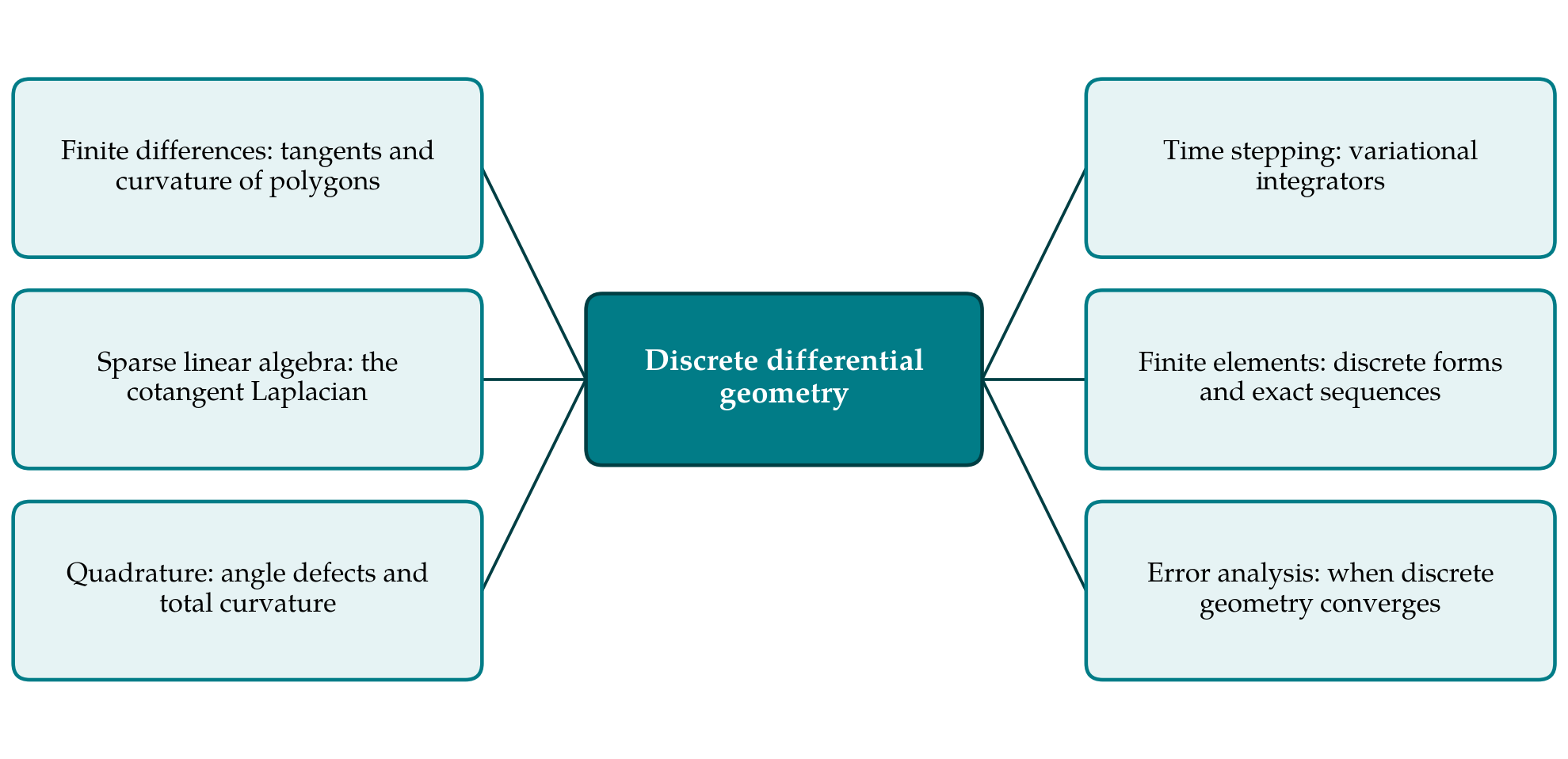
The cotangent formula for the Laplacian on a triangle mesh, used by Pinkall and Polthier (1993) to compute discrete minimal surfaces, is the best single example. It can be derived in a lecture as the gradient of the Dirichlet energy of a piecewise linear function, and it coincides with the stiffness matrix of linear finite elements. The matrix is sparse, symmetric and positive semidefinite, so it leads directly to the linear algebra of the course. Solving the heat equation with it for one implicit step, followed by a Poisson problem, yields geodesic distances on a surface (Crane et al., 2013b), an application that students can program in an afternoon and see on the screen. Figure 1 sketches how this and similar examples attach to the standard topics, and Table 1 lists concrete pairings.
| Standard topic | Discrete-geometric counterpart | What the student gains |
|---|---|---|
| Numerical differentiation | Turning angles and edge normals of a polygon | A consistent formula can also satisfy a theorem exactly |
| Quadrature | Angle defect and the discrete Gauss-Bonnet theorem | Integrated quantities may be exact when pointwise ones are not |
| Sparse linear systems | Cotangent Laplacian (Pinkall and Polthier, 1993) | Where sparse symmetric matrices come from |
| Initial value problems | Variational integrators (Marsden and West, 2001) | Long-time behaviour is not captured by order alone |
| Finite elements | Cochains and the discrete exterior derivative | Vector calculus identities as matrix identities |
| Convergence analysis | The Schwarz lantern | Pointwise convergence of a mesh does not imply convergence of area |
The discrete Gauss-Bonnet theorem serves the same purpose for quadrature. Define the curvature at a vertex of a closed triangulated surface as the angle defect, the amount by which the angles meeting there fall short of a full turn. The defects sum to the Euler characteristic of the surface multiplied by a full turn, exactly and for every triangulation. A student who verifies this on a coarse mesh of a torus has learned that topology constrains computation, a lesson otherwise postponed to graduate courses. The classical smooth statement, as found in do Carmo (1976), then appears as the limit of something already understood.
4. Objections
The first objection is that the syllabus is full. It is, and every proposal to add material must say what gives way. The examples above, however, are mostly substitutions. A lecture on numerical differentiation can use a polygon as its example at no extra cost, and the cotangent matrix can replace the five-point stencil as the model sparse system in one of several places. A single week devoted to the structural viewpoint, placed after ordinary differential equations, would suffice to state the principle and illustrate it.
The second objection concerns prerequisites: differential geometry is not usually required of students entering numerical analysis. The discrete theory needs less than this objection supposes. Angles, areas and normals of triangles are school geometry, and the smooth statements can be quoted as motivation without proof. The dependence arguably runs the other way, since students who have handled discrete curvature arrive at a later course in differential geometry with intuition that the smooth definitions alone seldom supply.
The third objection is the most serious. Discrete differential geometry can look like a collection of attractive formulas whose convergence is asserted and not proved, and the convergence theory is in fact subtle. Polyhedral surfaces can converge to a smooth surface pointwise while their areas and curvatures do not, as the Schwarz lantern shows, and convergence of the normals is the condition that restores order (Hildebrandt et al., 2006). Nor can any discrete Laplacian on general meshes have all the properties of the smooth one at once (Wardetzky et al., 2007). These facts are not reasons to exclude the subject. They are among the most instructive things a course could contain, because they show that consistency, structure and convergence are different properties that have to be established separately.
A last objection holds that the material belongs to computer graphics. The applications that made it prominent are indeed graphical, but the same constructions appear in elasticity, electromagnetism and fluid simulation, and the oldest of them, Regge's simplicial formulation of general relativity, is older than most of computer graphics (Regge, 1961).
5. Implications for Curriculum Design
If the argument is accepted, three levels of change are possible. The lightest is to replace selected examples and exercises with geometric ones, as in Table 1, leaving the list of topics untouched. The second is a short unit on structure preservation, with the turning-angle theorem, a symplectic method for the pendulum and the cotangent Laplacian as its three examples, and with the Schwarz lantern as a cautionary case. The third is an elective that follows the first course and takes discrete exterior calculus as its organizing idea, leading naturally towards finite element exterior calculus (Arnold et al., 2006). Which level suits a department depends on its students and its staff. Whether any of them improves learning is an empirical question that this article does not answer, and one that those who try the changes should examine and report.
Assessment would need to follow. Questions that ask only for the order of a method reward the approximation viewpoint alone. Asking which quantities a scheme conserves exactly, and why, tests the other half of the subject, and such questions are no harder to set or to mark.
6. Conclusion
Numerical analysis has absorbed the idea that good discretizations preserve structure, and its undergraduate teaching has not yet caught up. Discrete differential geometry offers the most concrete and least demanding route by which students can meet that idea: polygons whose turning angles sum exactly, meshes whose curvature knows their topology, and a Laplacian that is at once a geometric object, a finite element matrix and a sparse linear system. Giving these examples a place in the first course would cost little and would show students that accuracy is one measure of a numerical method, and faithfulness to structure another.
Conflict of interest
To be declared by the author(s) before publication.
Funding
To be declared by the author(s) before publication.