International Journal of Applied and Solid Mechanics

Identifying Hyperelastic Parameters of Soft Elastomers From Digital Image Correlation of Biaxial Tests

Seoyeon Muthukumar¹, Satoshi Guerrero², Magdalena Moreno³

¹ Department of Mechanical Engineering, Nejd University Centre for Mechanical Engineering, Tanzania, ² Department of Mechanical Engineering, Kaveri Academy of Mechanical Engineering, Kyrgyzstan, ³ Department of Mechanical Engineering, Pampas Institute of Mechanical Engineering, Belgium

Published 04 Jun 2026 Vol. 1, Article 3 10.62715/ijasm.2026.v1.i1.pp15-20 0 accesses 0 citations

Download PDF XML HTML EPUB

0Accesses

0Citations

Abstract

Soft elastomers such as silicones and natural rubber are modelled as hyperelastic solids whose behaviour is fixed by a strain energy function. The parameters of that function are commonly fitted to a uniaxial tension test, and models fitted in this way often predict other deformation states badly. Biaxial testing of a cruciform specimen explores a wider range of deformation, but the stress in the gauge region cannot be obtained from the measured forces alone because the field is not uniform. Digital image correlation supplies the missing information by measuring the displacement field over the whole specimen. This article proposes a seven-step procedure that combines the two: specimen and loading-path design, speckle preparation and stereo calibration, preconditioning and testing, computation of displacement fields with an estimate of measurement noise, selection of candidate strain energy functions, inverse identification by finite element model updating or the virtual fields method, and checks of identifiability with validation on a loading path not used for fitting. Each step is described with the choices it involves and the record it should leave. The procedure is assembled from established methods and published guidance. It is a proposal and has not been applied or validated in this article.

Keywords: Digital image correlation Hyperelasticity Biaxial testing Inverse identification Virtual fields method Elastomers

1. Introduction

Silicone rubbers, polyurethanes, natural rubber and hydrogels are used in seals, soft robots, biomedical devices and tissue phantoms, and each of these applications is designed with finite element models that treat the material as hyperelastic. A hyperelastic model is defined by a strain energy function, and its usefulness depends on the parameters put into it. The standard source of those parameters is still a dumbbell specimen pulled in uniaxial tension. Such a test visits one path in the space of deformations. A model fitted to it alone can reproduce that path closely and still be seriously wrong in equibiaxial or planar extension, as comparisons against the classical multi-mode data of Treloar (1944) have repeatedly shown (Marckmann and Verron, 2006).

The need for more than one deformation mode was understood early. Rivlin and Saunders (1951) stretched rubber sheets biaxially to probe how the strain energy depends on each of the two principal invariants. Homogeneous sheet tests of that kind are laborious, and modern biaxial machines instead load a cruciform specimen through four arms. The cruciform is convenient to grip and gives access to any ratio of the two in-plane stretches, but its stress field is heterogeneous: the arms shield the centre, and the stress there cannot be computed by dividing force by area. Full-field optical measurement, and digital image correlation in particular, changes the position. If the displacement is known everywhere on the surface, the heterogeneity becomes a source of information, and the parameters can be found by an inverse method (Avril et al., 2008).

This article sets out a procedure for doing so in an ordinary materials laboratory. It is written as a method: a sequence of steps, each with its reasoning. It is a proposal drawn from the literature and from published good-practice guidance, and it is not accompanied by an application to test data. What would be needed to validate it is stated near the end.

2. Background

The procedure rests on three bodies of established work: constitutive models for rubber-like solids, digital image correlation, and inverse identification from full-field data.

2.1. Strain energy functions and the fitting problem

For an isotropic, incompressible solid the strain energy can be written in terms of the first two invariants of the deformation or of the principal stretches (Holzapfel, 2000). The neo-Hookean model has one parameter and depends linearly on the first invariant. The form due to Mooney (1940), later generalised by Rivlin, adds the second invariant. Yeoh (1993) used a cubic polynomial in the first invariant only, the model of Ogden (1972) is a sum of powers of the principal stretches, and the models of Arruda and Boyce (1993) and Gent (1996) introduce a limiting chain extensibility to capture stiffening at large stretch. Flexible models fit one data set easily and can behave unphysically outside it. Ogden et al. (2004) demonstrated that least-squares fitting of such models is not unique, with several parameter sets giving nearly the same residual.

2.2. Digital image correlation

Digital image correlation tracks a random surface pattern between a reference image and deformed images and returns the displacement of small subsets of pixels. With one camera it measures in-plane motion of a flat specimen; with two calibrated cameras it measures shape and three-dimensional displacement, which removes the error caused by out-of-plane movement (Sutton et al., 2009; Pan et al., 2009). Strain is obtained by differentiating the displacement, an operation that amplifies noise and that depends on user settings: subset size, step and strain window. The good practices guide of the International Digital Image Correlation Society sets out how to choose and report them (Jones and Iadicola, 2018). Elastomers bring two special difficulties. The pattern must follow very large stretches without cracking or debonding, and thin specimens wrinkle or bulge if compressive stress develops anywhere.

2.3. Inverse identification

Two families of method dominate. Finite element model updating, which goes back to Kavanagh and Clough (1971), simulates the test with trial parameters and adjusts them until computed displacements and forces match the measured ones. It is general, tolerates incomplete fields and uses the same software as the eventual design analysis, but each iteration requires a nonlinear solution. The virtual fields method applies the principle of virtual work directly to the measured strain field with chosen test functions and needs no forward simulation (Pierron and Grédiac, 2012); Promma et al. (2009) applied it to a hyperelastic model of rubber using heterogeneous tests. It is fast, but it requires strains over the whole region considered and assumes a through-thickness state, usually plane stress, in order to pass from surface measurements to volume integrals.

3. The Proposed Procedure

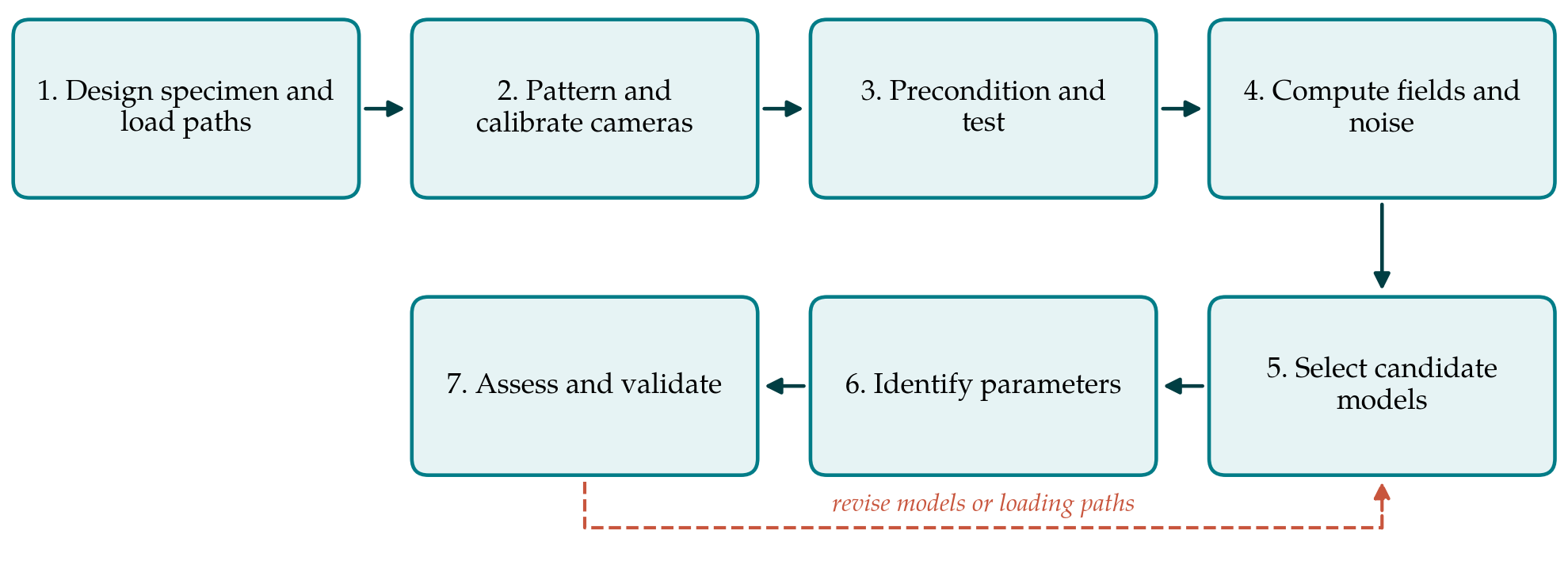
The proposed procedure has seven steps. Table 1 lists the output of each and the check applied before moving on, and Figure 1 shows the sequence, including the return path taken when identification fails its checks.

Table 1: Steps of the proposed identification procedure, with the output of each and the check made before the next step
Step	Main output	Check before proceeding
1. Design specimen and paths	Cruciform geometry and a set of load ratios	Simulated field spans distinct deformation modes
2. Pattern and calibrate	Speckled specimen and calibrated stereo rig	Calibration residual and static noise acceptable
3. Precondition and test	Synchronised images and arm forces for each path	Repeat cycles overlap after preconditioning
4. Compute fields	Displacement and stretch maps with a noise estimate	Field symmetry and balance of arm forces
5. Select candidate models	Short list of strain energy functions	Each model admissible over the tested range
6. Identify parameters	Parameter set and residual for each model	Same optimum from several starting points
7. Assess and validate	Confidence bounds; prediction of the held-out path	Prediction error within measurement uncertainty

Figure 1: Sequence of the proposed procedure, with the return path taken when validation fails

3.1. Step 1: Design the specimen and the loading paths

The specimen should produce a field rich enough to separate the parameters and should not fail in the arms before the centre has stretched appreciably. A cruciform with generous fillet radii, and where necessary slits along the arms to reduce their transverse stiffness, is a common starting point. Before any material is cut, the test is simulated with literature values for a comparable elastomer, and the simulated field is examined on a plot of the two principal stretches: points should spread between the uniaxial, planar and equibiaxial lines. At least three loading paths are planned, typically equibiaxial, one arm pair held while the other is extended, and an intermediate ratio. One path is set aside for validation and plays no part in fitting.

3.2. Step 2: Apply the pattern and calibrate the cameras

A stereo arrangement is preferred because thin elastomer sheets rarely stay flat. The speckle pattern is applied with a paint or powder that stretches with the surface; for very large stretch the pattern is best made from discrete particles, so that speckles separate without cracking. Feature size should span several pixels at the chosen magnification and remain resolvable when the surface area has multiplied. The cameras are calibrated with a target that fills the field of view, and a set of images of the unloaded specimen is recorded. Correlating those static images against each other gives the noise floor of displacement and strain for the actual set-up (Jones and Iadicola, 2018).

3.3. Step 3: Precondition and run the tests

Filled elastomers soften during the first loading cycles to a given stretch, the effect reviewed by Mullins (1969), and virgin and cycled materials are in effect different materials. The procedure therefore fixes in advance which state is to be characterised. For the stabilised state, each specimen is cycled several times to the maximum stretch of the path before images are recorded, and a fresh specimen is used for each path, since softening depends on the deformation history. Tests are run slowly enough for rate effects to be small, which is verified by repeating one path at a different rate. Forces in all four arms are logged in step with the images.

3.4. Step 4: Compute the fields and their uncertainty

Images are correlated with settings chosen from the noise study, and the reference image is updated incrementally where stretches are too large for a single reference. The outputs are displacement maps and, by differentiation, the in-plane deformation gradient, from which the principal stretches follow; the through-thickness stretch is obtained from incompressibility. Two checks are made. The fields should show the symmetries of the specimen, and departures indicate misalignment or slipping grips. The opposing arm forces should balance. Regions near grips and free edges, where correlation is poor, are masked, and the mask is recorded.

3.5. Step 5: Select candidate models

Candidate strain energy functions are chosen before fitting and kept few. A reasonable short list contains the neo-Hookean model as a baseline, a two-parameter form with second-invariant dependence, the Yeoh model, a low-order Ogden model and one limiting-extensibility model. The comparative study of Marckmann and Verron (2006) is a useful guide to how each behaves across deformation modes. For every candidate the admissible parameter range is written down, so that the optimiser cannot return a set that violates stability requirements within the tested stretches.

3.6. Step 6: Identify the parameters

Either inverse route can be used, and using both on the same data is a strong cross-check. In finite element model updating, the measured boundary displacements at the edge of the region of interest are imposed on a model of that region, and the cost function combines the mismatch in interior displacements with the mismatch in arm forces, each scaled by its measurement uncertainty. Without the force term the parameters are determined only up to a common factor, because kinematics alone carry no stress scale. In the virtual fields method, virtual fields are chosen so that the measured forces enter the external virtual work, and the resulting equations are solved by least squares over all images. The optimisation is started from several well-separated initial guesses.

3.7. Step 7: Assess identifiability and validate

A low residual does not show that the parameters are known. Sensitivity of the cost function to each parameter is evaluated at the optimum, and strong correlation between parameters, or a flat direction in the cost surface, is reported as such. Confidence bounds can be estimated by repeating the identification on fields perturbed with noise at the measured level. The identified models are then used to predict the held-out loading path, and the predicted forces and fields are compared with those measured. If no candidate predicts it within the measurement uncertainty, the loop in Figure 1 is followed: the model list or the loading paths are revised.

4. Fitting the Procedure to the Laboratory

The procedure assumes a biaxial frame with independent control of two axes and a stereo correlation system. Where only a uniaxial frame exists, much of the benefit can be kept by testing a specimen with a deliberately heterogeneous shape, such as a wide strip with a hole, and applying steps 2 to 7 unchanged; the range of biaxiality will be narrower and the identifiability checks become more important. Compressible foams and gels need a volumetric term and a measurement of thickness change, which stereo correlation on both faces or a separate confined compression test can provide. For strongly rate-dependent or anisotropic materials the isotropic hyperelastic framework is insufficient, and the procedure then describes only the equilibrium response it is designed around.

5. Limitations and What Remains to Be Shown

The procedure is proposed and has not been validated here. Its components are established individually, but their combination into the sequence above has not been tested in this article on any material. Three demonstrations would be needed. The first is recovery of known parameters from synthetic images, generated by deforming a speckle pattern with a simulated field and adding realistic noise, which tests the chain from correlation to identification without material uncertainty. The second is agreement, on a real elastomer, between parameters from this procedure and those from conventional homogeneous tests in uniaxial, planar and equibiaxial modes. The third is reproducibility between laboratories using different equipment.

Some limitations are inherent. Surface measurement cannot see through-thickness variation, and the plane stress assumption weakens near fillets in thick specimens. Maximum stretch at the centre of a cruciform is usually well below the failure stretch of the material, since the arms fail first, so parameters governing the stiffening regime may be poorly determined; a uniaxial test to large stretch can be added to the data to cover it. Viscoelasticity and the Mullins effect are excluded by protocol and not modelled. And the outcome is conditional on the list of candidate models: the procedure ranks the candidates given to it and cannot show that a better function does not exist.

6. Conclusion

Parameters for hyperelastic models of soft elastomers are more trustworthy when they are identified from several deformation modes at once, and a cruciform biaxial test observed by digital image correlation offers those modes in a single specimen. The seven steps proposed here arrange established techniques so that each feeds the next and leaves a checkable record: a simulated design, a measured noise floor, preconditioned tests, masked and verified fields, a declared model list, inverse identification with force information, and validation on an unused path. Whether the procedure delivers the accuracy it aims for remains to be demonstrated by the synthetic and experimental tests outlined above.

Conflict of interest

To be declared by the author(s) before publication.

Funding

To be declared by the author(s) before publication.

References

[1] Arruda, E.M. and Boyce, M.C. A three-dimensional constitutive model for the large stretch behavior of rubber elastic materials. Journal of the Mechanics and Physics of Solids https://doi.org/10.1016/0022-5096(93)90013-6 41(2), 389-412 (1993).
[2] Avril, S., Bonnet, M., Bretelle, A.-S., Grédiac, M., Hild, F., Ienny, P., Latourte, F., Lemosse, D., Pagano, S., Pagnacco, E. and Pierron, F. Overview of identification methods of mechanical parameters based on full-field measurements. Experimental Mechanics https://doi.org/10.1007/s11340-008-9148-y 48(4), 381-402 (2008).
[3] Gent, A.N. A new constitutive relation for rubber. Rubber Chemistry and Technology https://doi.org/10.5254/1.3538357 69(1), 59-61 (1996).
[4] Holzapfel, G.A. Nonlinear Solid Mechanics: A Continuum Approach for Engineering. Wiley, Chichester (2000).
[5] Jones, E.M.C. and Iadicola, M.A. (eds.) A Good Practices Guide for Digital Image Correlation. International Digital Image Correlation Society https://doi.org/10.32720/idics/gpg.ed1 (2018).
[6] Kavanagh, K.T. and Clough, R.W. Finite element applications in the characterization of elastic solids. International Journal of Solids and Structures https://doi.org/10.1016/0020-7683(71)90015-1 7(1), 11-23 (1971).
[7] Marckmann, G. and Verron, E. Comparison of hyperelastic models for rubber-like materials. Rubber Chemistry and Technology https://doi.org/10.5254/1.3547969 79(5), 835-858 (2006).
[8] Mooney, M. A theory of large elastic deformation. Journal of Applied Physics https://doi.org/10.1063/1.1712836 11(9), 582-592 (1940).
[9] Mullins, L. Softening of rubber by deformation. Rubber Chemistry and Technology https://doi.org/10.5254/1.3539210 42(1), 339-362 (1969).
[10] Ogden, R.W. Large deformation isotropic elasticity: On the correlation of theory and experiment for incompressible rubberlike solids. Proceedings of the Royal Society of London A https://doi.org/10.1098/rspa.1972.0026 326(1567), 565-584 (1972).
[11] Ogden, R.W., Saccomandi, G. and Sgura, I. Fitting hyperelastic models to experimental data. Computational Mechanics https://doi.org/10.1007/s00466-004-0593-y 34(6), 484-502 (2004).
[12] Pan, B., Qian, K., Xie, H. and Asundi, A. Two-dimensional digital image correlation for in-plane displacement and strain measurement: A review. Measurement Science and Technology https://doi.org/10.1088/0957-0233/20/6/062001 20(6), 062001 (2009).
[13] Pierron, F. and Grédiac, M. The Virtual Fields Method: Extracting Constitutive Mechanical Parameters from Full-field Deformation Measurements. Springer, New York (2012).
[14] Promma, N., Raka, B., Grédiac, M., Toussaint, E., Le Cam, J.-B., Balandraud, X. and Hild, F. Application of the virtual fields method to mechanical characterization of elastomeric materials. International Journal of Solids and Structures 46(3-4), 698-715 (2009).
[15] Rivlin, R.S. and Saunders, D.W. Large elastic deformations of isotropic materials VII. Experiments on the deformation of rubber. Philosophical Transactions of the Royal Society of London A https://doi.org/10.1098/rsta.1951.0004 243(865), 251-288 (1951).
[16] Sutton, M.A., Orteu, J.-J. and Schreier, H.W. Image Correlation for Shape, Motion and Deformation Measurements: Basic Concepts, Theory and Applications. Springer, New York (2009).
[17] Treloar, L.R.G. Stress-strain data for vulcanised rubber under various types of deformation. Transactions of the Faraday Society https://doi.org/10.1039/TF9444000059 40, 59-70 (1944).
[18] Yeoh, O.H. Some forms of the strain energy function for rubber. Rubber Chemistry and Technology https://doi.org/10.5254/1.3538343 66(5), 754-771 (1993).

Article metrics

0 total accesses since publication. 0 citing articles have been indexed to date.