1. Introduction
A carbide insert wears from the first second of cutting. Abrasion and adhesion grind a flat land on the flank, diffusion and chemical wear hollow a crater on the rake face, and at some point the edge either reaches a wear limit that spoils size and finish or fractures outright (Trent and Wright, 2000). The relation between cutting speed and life has been known since Taylor (1907), but life scatters widely about any such law, because workpiece hardness, stock allowance, coolant delivery and the insert itself vary from part to part. A fixed tool-change count is therefore set conservatively, and a good share of usable edge life is thrown away.
Monitoring the tool in process has been a research subject for more than forty years. The reviews prepared for the International Academy for Production Engineering describe the sensors available, namely dynamometers, accelerometers, acoustic emission transducers and current or power sensors, together with the signal processing and decision methods applied to them (Byrne et al., 1995; Teti et al., 2010). Uptake in ordinary job shops has been slow. A force dynamometer is costly and alters the stiffness of the setup; an acoustic emission sensor has to be mounted close to the cut and survives poorly among chips and coolant; and each needs its own data acquisition (Dimla, 2000; Li, 2002).
Spindle drive power is the exception. It is measured inside the drive for control purposes, it costs nothing to install, and nothing has to be placed in the work area. Its drawbacks are equally well known: the signal is filtered by the inertia of the spindle, it contains friction and electrical losses, and it reflects every change in cutting load whether or not wear is the cause. This article proposes a procedure that works within those limits. It is a methodological proposal and reports no trials.
2. Background
The physical basis is simple. Cutting power is the product of the tangential cutting force and the cutting speed. For a sharp tool the force can be estimated from the uncut chip cross-section and a specific cutting force that depends on the work material and falls slowly with chip thickness, the relation introduced by Kienzle (1952) and found in every machining textbook (Altintas, 2012). As the flank land grows, rubbing between land and workpiece adds a force component that increases with the width of the land. All three force components rise, the feed and radial components proportionally more than the tangential one, which is why feed drive current has also been studied as a source of force information (Altintas, 1992).
Stein and Wang (1990) analysed power monitoring on induction motor drives and showed how the measured power relates to torque at the tool once losses and the dynamics of the drive are accounted for. Shao et al. (2004) built a cutting power model for face milling that includes a flank wear term and used it to follow wear from spindle power. Reviews of indirect monitoring list motor current and power among the more robust and least intrusive signals, while noting their limited bandwidth and their weakness on small tools, where cutting power is a small fraction of the idle power of the spindle (Rehorn et al., 2005).
On the decision side, much of the literature has trained neural networks or other learning models on many signal features. Sick (2002) reviewed more than a decade of such work in turning and found that many studies gave little attention to how their models generalise beyond the conditions used for training. The procedure below therefore favours a small number of physically meaningful quantities and a model simple enough to be recalibrated by shop staff.
3. The Proposed Procedure
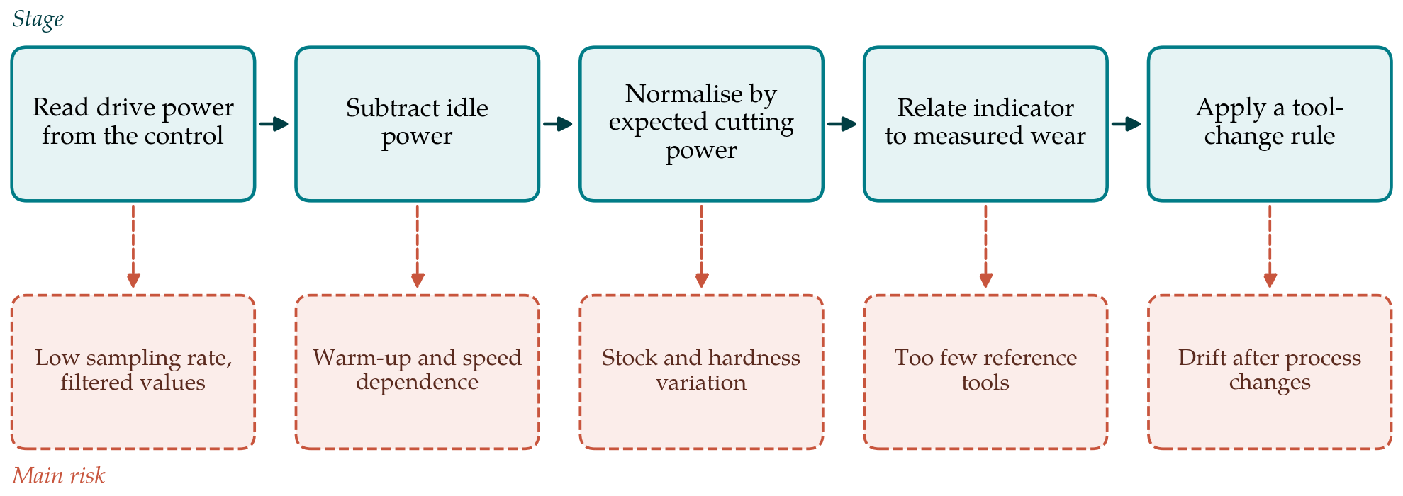
The procedure has five stages, each with a characteristic risk; Figure 1 sets them side by side. The stages are taken in order in the subsections that follow.
3.1. Stage 1: Access and qualify the signal
Current controls publish spindle load, drive power or torque-producing current as data items that can be read over open interfaces such as MTConnect (MTConnect Institute, 2018) or the OPC UA companion specifications for machine tools. Three things have to be established before the value is used. One is its meaning: whether it is electrical power, a percentage of rated load or a current, and how it is filtered. A second is its sampling interval, which on many controls is tens or hundreds of milliseconds and is adequate for the mean power of a cut but not for tooth-by-tooth detail. The third is its context: the same data stream must supply the active tool number, the program block, the spindle speed and the feed rate, so that power can be attributed to a tool and an operation.
3.2. Stage 2: Characterise idle power
Net cutting power is the measured power less what the spindle draws when running free. Idle power depends on speed and falls as bearings and lubricant warm up. It is characterised by running the spindle unloaded across the speed range, cold and warm, and is then refreshed automatically in production from the air-cut interval that precedes each engagement, when the spindle is at speed and the tool has not yet touched the work. Using the air cut of the same pass as the reference removes most of the thermal drift. Acceleration and deceleration intervals are discarded.
3.3. Stage 3: Segment and normalise
Raw net power rises with wear but also with depth of cut, feed, speed and material. To separate these, each cutting segment is divided by the power expected for a sharp tool under the programmed conditions. The expected value is the material removal rate multiplied by the specific cutting energy from the Kienzle relation, with the chip thickness taken from the feed and the tool geometry. The ratio of measured to expected power is dimensionless and is close to a constant for a sharp edge. In practice the constant is not exactly one, because handbook coefficients and drive efficiency are approximate, so the ratio is referred to its own value over the first parts cut with each new edge. Table 1 lists the influences other than wear that move spindle power and how the procedure treats each.
| Influence | Effect on the signal | Treatment |
|---|---|---|
| Spindle warm-up | Idle power falls over the first period of running | Idle reference taken from the air cut of each pass |
| Programmed speed, feed and depth | Cutting power scales with removal rate | Division by expected power from the force model |
| Stock allowance variation | True depth differs from programmed depth | Use finishing passes; average over several parts |
| Workpiece hardness | Specific cutting energy shifts between batches | Re-reference the ratio at each new edge and batch |
| Coolant condition | Friction and built-up edge change the force | Record coolant state; treat changes as a new regime |
| Drive filtering and losses | Signal lags and understates short peaks | Use mean power over steady segments only |
Segments are kept only where the cut is steady: constant programmed conditions for long enough that the filtered signal has settled. Operations in which the cutting power is small compared with idle power, such as light finishing with small tools on a large spindle, should be identified at this stage and left out of scope, since no later processing can recover a signal that is buried in the losses.
3.4. Stage 4: Calibrate against measured wear
The indicator is the normalised power ratio of each segment relative to the new-edge reference, smoothed over consecutive parts. To relate it to wear, a commissioning period is needed in which inserts are removed at intervals and the flank wear land is measured under a toolmaker's microscope, following the definitions and criteria of the tool-life testing standards for turning (ISO, 1993) and milling (ISO, 1989). Several edges should be followed from new to the wear criterion, so that the scatter between edges is visible.
The relation between indicator and wear land is then fitted with a simple monotone model, a straight line or a low-order curve, and its uncertainty is estimated by leaving out one whole edge at a time and predicting it from the others. Leaving out whole edges, and not individual observations, is essential; observations from the same edge are strongly correlated, and a random split gives a flattering and false picture of accuracy, the general hazard described in the statistical learning literature (Hastie et al., 2009). If the prediction error across edges is too large for a tool-change decision, the operation is not a candidate for power-based monitoring and the procedure should say so.
3.5. Stage 5: Apply a tool-change rule and watch for drift
In production the fitted relation is inverted: the tool is flagged for change when the predicted wear, plus a margin reflecting the calibration uncertainty, reaches the criterion. A second, independent rule guards against breakage, using a short-term jump or collapse in power, as commercial monitoring systems do (Jemielniak, 1999). The count-based limit is kept as a backstop until confidence has been built. Drift is checked by measuring an occasional insert at removal and comparing its wear with the prediction.
4. Fitting the Procedure to a Shop
The procedure suits repetitive work best: turning or milling of one part family in batches, where the same operation recurs often enough for a reference to be built and where the cut is long and heavy enough for cutting power to stand clear of the idle level. One-off work, short interrupted cuts and small-diameter tools do not. The commissioning measurements are the real cost.
5. Limitations and What Remains to Be Shown
This article sets out a procedure and does not demonstrate it. Its usefulness depends on quantities that only trials can supply: how large the rise in normalised power is between a new edge and the wear criterion for common insert and material pairs, how that rise compares with the part-to-part scatter caused by stock and hardness, and how well a calibration transfers across machines of the same type. A validation study should report prediction error on edges not used for fitting, the number of false and missed tool-change flags against microscope measurement, and the edge life recovered compared with the count-based rule.
Some limits are inherent. Power responds mainly to flank wear and is a poor guide to crater wear, notching or the small chipping that damages surface finish before the load changes noticeably.
6. Conclusion
Spindle power is a modest signal, but it is present on every machine and needs no hardware. The procedure proposed here tries to extract what it can honestly give: a normalised load indicator, tied to measured flank wear through a short commissioning study, and used with a margin and a backstop. Establishing where the approach is accurate enough to replace count-based tool changes is an empirical task for which the necessary measurements have been specified.
Conflict of interest
To be declared by the author(s) before publication.
Funding
To be declared by the author(s) before publication.