1. Introduction
Tropical forest is increasingly a landscape of fragments: patches of a few hectares to a few thousand, set in pasture, oil palm, tea or smallholder farms. Deciding which patches still hold a rich bird community, and whether corridors or replanting change that, requires surveys at many sites and repeated over years. Point counts by expert observers remain the reference method, but observers able to identify several hundred species by voice are few, and their time is the limiting cost of most tropical surveys.
Passive acoustic monitoring removes part of that constraint. Small programmable recorders such as the AudioMoth can be left at a site for weeks and cost little enough to deploy by the dozen (Hill et al., 2018). The difficulty moves to analysis, since no one can listen to thousands of hours of sound. Acoustic indices were devised as a shortcut: summary statistics of the distribution of sound energy across time and frequency, intended to rise and fall with the diversity of animals calling (Sueur et al., 2008; Sueur et al., 2014).
This article sets out a protocol for using such indices to estimate bird species richness across forest fragments in the tropics. It takes the view that an index is a predictor to be calibrated locally against known richness, and builds the calibration and its validation into the procedure. The protocol is a proposal drawn from published methods. It is not applied to recordings here and has not been validated.
2. Background
Soundscape ecology treats the sound of a place as the sum of biological sources (biophony), physical sources such as wind and rain (geophony) and human sources (anthrophony) (Pijanowski et al., 2011). Indices try to isolate properties of the first. Table 1 lists the six in most common use, with what each measures and what is known to distort it.
| Index | What it measures | Main confounds | Source |
|---|---|---|---|
| Acoustic Complexity (ACI) | Variation in intensity between adjacent time steps within frequency bins | Rain; pulsed insect song | Pieretti et al., 2011 |
| Acoustic Entropy (H) | Evenness of energy across time and across the spectrum | Broadband noise; silence | Sueur et al., 2008 |
| Bioacoustic Index (BI) | Area under the spectrum above its minimum within a set band | Loud single species; cicadas | Boelman et al., 2007 |
| Acoustic Diversity (ADI) | Shannon diversity of occupied frequency bands | Amplitude threshold; insect bands | Villanueva-Rivera et al., 2011 |
| Acoustic Evenness (AEI) | Gini coefficient of occupied frequency bands | Amplitude threshold; insect bands | Villanueva-Rivera et al., 2011 |
| Normalised Difference Soundscape (NDSI) | Ratio of energy in a biological band to a human-noise band | Low-pitched birds; high-pitched machinery | Kasten et al., 2012 |
Tests of the indices against bird richness have given mixed results. In a comparison of temperate sites in England with tropical sites in Ecuador, indices predicted avian richness in the former and not in the latter (Eldridge et al., 2018). Work in two regions of Yunnan found correlations with bird diversity that were weak and differed between regions (Mammides et al., 2017). A meta-analysis of the published tests reported a positive overall relation between indices and diversity that was only moderate in strength and highly variable among studies (Alcocer et al., 2022).
The reasons are understood in outline. In tropical forest, cicadas, katydids and frogs often produce more acoustic energy than birds, and they do so in bands that overlap bird song. Heavy rain saturates every index. A single loud species near the microphone can dominate. Indices also respond to the settings used to calculate them, and default settings were chosen for other ecosystems. Metcalf et al. (2021) showed for Amazonian forest that indices tracked biodiversity better when computed within frequency bands and times of day that matched the animals of interest. Several studies indicate that combinations of indices fitted with flexible models predict biological variables better than any one index (Buxton et al., 2018). In fragmented forest in eastern Australia, indices differed widely in how well they reflected landscape configuration and ecological condition (Fuller et al., 2015), a further sign that calibration cannot be skipped.
3. The Proposed Protocol
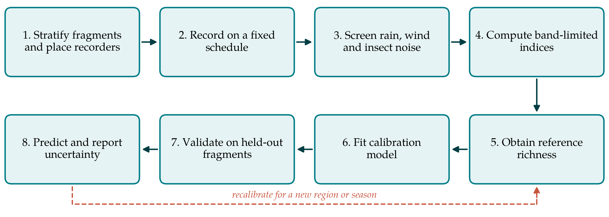
The protocol has eight steps, shown in Figure 1. The first three concern how recordings are gathered and cleaned, the fourth the indices, and the last four the calibration against reference data and its use.
3.1. Step 1: Stratify fragments and place recorders
Fragments are grouped by the variables the survey is meant to examine, usually area, isolation from continuous forest and the type of surrounding land use, and sampled within each group so that the calibration spans the full range of conditions. Continuous forest sites are included as the upper reference. Within a fragment, recorders are placed at several points, including interior and edge, at a fixed height on a trunk, facing away from streams and roads. Points are spaced widely enough that the same birds are not recorded twice; a few hundred metres is usual in closed forest. All recorders are of one model with one gain setting, because index values are not comparable across devices with different microphone responses.
3.2. Step 2: Record on a fixed schedule
A sampling rate of 48 kHz captures sound up to 24 kHz, which covers the vocal range of nearly all birds and leaves headroom for filtering. Continuous recording is seldom affordable in battery and storage, so a duty cycle is used, for example one minute in every ten through the day and night. Guidelines derived from tropical forest recordings stress that indices vary strongly with time of day and that a site needs many hours of recording, spread over many days, before its index values settle (Bradfer-Lawrence et al., 2019). Recorders at all sites should run over the same dates, or in rotations balanced across fragment groups, so that weather and season are not confounded with fragment type.
3.3. Step 3: Screen rain, wind and insect noise
Each recording is screened before any index is calculated. Minutes with heavy rain or strong wind are identified, either from a nearby rain gauge or from the recordings themselves, since rain produces broadband energy with a characteristic flat spectrum, and are set aside. Persistent narrow-band insect choruses are noted with their frequency limits. Files with recorder faults or handling noise are removed. The proportion of minutes excluded is recorded for each site, because it is itself informative and because uneven exclusion could bias the comparison.
3.4. Step 4: Compute band-limited indices
The six indices of Table 1 are calculated for each retained minute. They are computed twice: over the full spectrum, and within a band chosen from the regional avifauna, typically from about 1 kHz up to the lower edge of the dominant cicada band where one exists. Values are then summarised for each site within ecologically defined windows, at least the dawn chorus, mid-morning and dusk, using the median and a measure of spread. Following Metcalf et al. (2021), the band-limited, dawn-window values are expected to carry most of the information about birds, and the remaining values help the model discount insects and noise. The software, its version and every setting are recorded.
3.5. Step 5: Obtain reference richness
Calibration needs an independent estimate of bird richness at a subset of recorder points. Two sources are combined. Standard point counts of fixed duration are made at the recorder by an experienced observer on several mornings. A random sample of recorded minutes from the same points, stratified by time of day, is annotated by an expert listener, who lists every species heard. Automated classifiers such as BirdNET (Kahl et al., 2021) can propose candidate species to speed the annotation, but their output is checked by ear, because coverage and accuracy for tropical species are uneven. Since richness rises with effort, the reference value for each point is expressed for a fixed number of counts or annotated minutes, using rarefaction where effort differs.
3.6. Step 6: Fit the calibration model
Reference richness is modelled as a function of the summarised indices. A random forest (Breiman, 2001) suits the task, since it handles correlated predictors and non-linear responses and has few settings. A generalised linear model with a small number of indices chosen in advance is fitted alongside it as a more transparent comparison. Predictors include the full-band and band-limited indices by time window and the proportion of minutes excluded for noise. Habitat variables are deliberately left out, so that the model's skill reflects the sound and not the map.
3.7. Step 7: Validate on held-out fragments
Recorder points within one fragment share birds, weather and background noise, so random cross-validation over points would overstate accuracy. Whole fragments are therefore held out in turn, the model is fitted to the rest, and predictions are compared with reference richness in the held-out fragment, as recommended for spatially structured data (Roberts et al., 2017). The prediction error and the rank correlation between predicted and reference richness are reported. A decision rule is fixed before the analysis: if the model cannot rank held-out fragments better than fragment area alone does, the indices are not used for estimation in that landscape.
3.8. Step 8: Predict and report uncertainty
A model that passes validation is applied to recorder points without reference data. Predictions are given with intervals derived from the validation error, and fragments are compared by class of richness (for example lower, middle and upper thirds) where the intervals do not support finer distinctions. The report states the region and season of calibration. A model is not carried to another region, forest type or season without new reference data, which is the feedback loop in Figure 1.
4. Fitting the Protocol to Practice
The reference data are the costly element, and their scale should be decided first. A workable division is to collect reference richness at roughly a third of the recorder points, chosen to span all fragment groups, and to use the remainder for prediction. Annotation effort is better spent on many short samples from many mornings than on long stretches of a few. Where an expert listener is available only briefly, recordings allow the annotation to be done later and elsewhere, and a second listener can check a sample to measure agreement. Raw audio should be archived, since learned acoustic features and species classifiers are improving quickly and old recordings can be reanalysed.
5. Limitations and What Remains to Be Shown
The protocol has not been tested, and the central uncertainty is whether calibrated indices will predict richness in a given tropical landscape at all. The published record gives grounds for doubt (Eldridge et al., 2018; Alcocer et al., 2022). The decision rule in the seventh step exists for that reason, and a negative result from it is a legitimate and publishable outcome. Even a successful calibration estimates the richness of species that vocalise during the recording windows. Quiet, rare and seasonally silent species are missed by indices and point counts alike.
Two further matters are unresolved. Fragmentation alters the soundscape through routes other than bird richness: edges are windier, closer to roads and often richer in generalist insects, so an index may track edge effects that happen to correlate with bird loss in the calibration set and fail elsewhere. Also, richness is a blunt target, because a fragment can keep its species count while forest specialists are replaced by common open-country birds. Indices cannot detect that turnover. Species-level classifiers can, and as they mature for tropical faunas the role of indices may narrow to rapid screening.
6. Conclusion
Acoustic indices are cheap to compute and tempting to over-interpret. For fragmented tropical forest, the published evidence supports their use only as locally calibrated predictors, restricted to the bands and hours in which birds dominate, combined in a multi-index model, and tested on fragments the model has not seen. The eight-step protocol proposed here arranges those requirements in a sequence that a survey team can follow and document. Whether it yields useful estimates is an empirical matter for each landscape, and the protocol is designed so that a team finds out before relying on the numbers.
Conflict of interest
To be declared by the author(s) before publication.
Funding
To be declared by the author(s) before publication.