1. Introduction
Soil water content is among the most useful variables a farm or a hydrological study can measure, and it has to be measured in many places because it varies over short distances (Robinson et al., 2008). Wireless nodes with buried probes are the obvious instrument. The early agricultural deployments showed how much can go wrong with them. The potato field pilot described by Langendoen et al. (2006) is a frank record of nodes that reset, drained their batteries and returned little data, and later guidance drawn from alpine deployments reads as a list of the same lessons learned again (Barrenetxea et al., 2008).
Many nodes in use today began as prototypes on a development board, with a general-purpose regulator, a sensor that is always powered and firmware that sleeps lightly. Such a design can last a season. It will not last five years, the horizon over which the cost of visiting a remote site to change batteries starts to dominate the cost of the hardware. Reaching that horizon rarely needs exotic components. It needs the existing design to be examined methodically and every microampere and every ingress path accounted for.
This article sets out a procedure for that examination. It is addressed to engineers who already have a working node and want to extend its service life, and it is written as a proposal: a sequence of steps with their rationale, drawn from published experience and standard practice. No node has been redesigned or deployed as part of this work, and no measurements are reported.
2. Background
Three areas of prior work inform the procedure: where the energy of a sensor node goes, what the sensing principle demands, and what the battery can actually deliver.
2.1. Energy use in duty-cycled nodes
A sensor node spends nearly all of its life asleep. Raghunathan et al. (2002) established the basic accounting: the radio dominates active consumption, and lifetime is governed by the duty cycle and by the current drawn while idle. Hardware built for the purpose, such as the Telos platform, was designed around a very low sleep current and a fast wake-up (Polastre et al., 2005). In long deployments the sleep term often turns out to be the larger one. The habitat monitoring study of Szewczyk et al. (2004) reported node lifetimes and failures that a simple active-time budget would not have predicted, which is an argument for modelling every state of the node and not only the obvious ones (Martinez et al., 2015).
Low-power wide-area radio has changed the communication side of the budget. A LoRaWAN class A device transmits when it has data, opens two short receive windows and is otherwise silent (LoRa Alliance, 2017), so it needs no synchronisation with neighbours and no routing duties (Raza et al., 2017). The energy per message depends strongly on the spreading factor, because a higher factor lengthens the time on air (Augustin et al., 2016; Casals et al., 2017). Regional duty-cycle regulations and the capacity of a gateway also limit how often a node may report (Adelantado et al., 2017).
2.2. Soil moisture sensing
Electromagnetic sensors infer water content from the dielectric permittivity of the soil, which rises steeply with moisture because the permittivity of water is far higher than that of mineral particles or air. Topp et al. (1980) gave the empirical relation that underlies time domain reflectometry. Low-cost capacitance probes work at lower frequencies and are more sensitive to soil temperature, salinity and texture; the evaluation by Bogena et al. (2007) documents these effects for one widely used probe and shows that corrections are needed. For the node designer two points follow. The probe needs a defined settling time after power is applied before its output is valid, and a supply that sags during the reading produces an error in the measurement itself.
2.3. Primary batteries for long deployments
Lithium thionyl chloride cells are the usual choice for multi-year unattended operation. They have a nominal voltage of 3.6 V, high energy density, a wide temperature range and very low self-discharge (Linden and Reddy, 2002). The low self-discharge comes from a passivation layer on the lithium anode, and the same layer causes a transient voltage drop when a cell that has rested is asked for a current pulse. Bobbin-type cells, which offer the highest capacity, are also limited in the pulse current they can supply. Rated capacity is quoted at a favourable discharge rate and temperature, and the capacity available in a cold field under pulsed load is lower. Energy harvesting is an alternative route to long life (Jiang et al., 2005) but adds a panel, a storage element and their own failure modes; the procedure here assumes a primary cell.
3. The Proposed Procedure
The procedure has eight steps, listed in Table 1 with the record that each should leave. Steps 1 to 3 establish the target, steps 4 to 7 change the design, and step 8 checks it. The procedure is proposed and has not been validated here.
| Step | What is done | Record produced |
|---|---|---|
| 1. Mission profile | Fix lifetime, reporting interval, temperature range and data loss tolerated | One-page requirements sheet |
| 2. Energy audit | List every state of the present node with its current and duration | State table and charge per day |
| 3. Budget | Derate cell capacity and divide by service hours to get average current | Budget with stated derating factors |
| 4. Sensing chain | Gate probe power, define settling time, validate readings | Timing diagram and plausibility rules |
| 5. Radio policy | Choose data rate handling, payload, confirmation and retry limits | Charge per uplink at each data rate |
| 6. Sleep state | Remove quiescent and leakage paths; select regulator and timer | Sleep current target by component |
| 7. Field hardening | Enclosure, cable entry, coating, pulse support for the cell | Environmental design checklist |
| 8. Verification | Profile current over full cycles; plan in-field health telemetry | Measured profile against budget |
3.1. Step 1: Fix the mission profile
The redesign starts from a written statement of what the node must do: the service life, the interval between readings, the temperature range at the site, the radio coverage expected, and how much data loss the application tolerates. The reporting interval deserves scrutiny. Soil moisture at rooting depth changes slowly except after rain or irrigation, so a long default interval with event-driven reports on rapid change is often adequate, and the choice multiplies through every later step.
3.2. Step 2: Audit the existing design
Each operating state of the present node is listed with the current it draws and the time spent in it per day: sleep, wake-up, sensor warm-up, conversion, radio transmit at each data rate in use, receive windows, and any housekeeping. Datasheet figures are a starting point, and measured values should replace them, since board-level leakage does not appear in any datasheet. The product of current and time in each state gives the daily charge, and the table shows at once which states matter.
3.3. Step 3: Derive the energy budget
The budget follows from the cell. Usable capacity is the rated capacity reduced for temperature, for pulsed discharge, for self-discharge over the service life and for the cut-off voltage at which the regulator and radio stop working. Five years is about 43,800 hours, so the permitted average current is the usable capacity divided by that figure. As a matter of arithmetic, a cell from which 5 Ah can be drawn supports an average of roughly 114 μA. The derating factors are judgements and should be written down with their sources, so that they can be revised when field evidence arrives.
3.4. Step 4: Rework the sensing chain
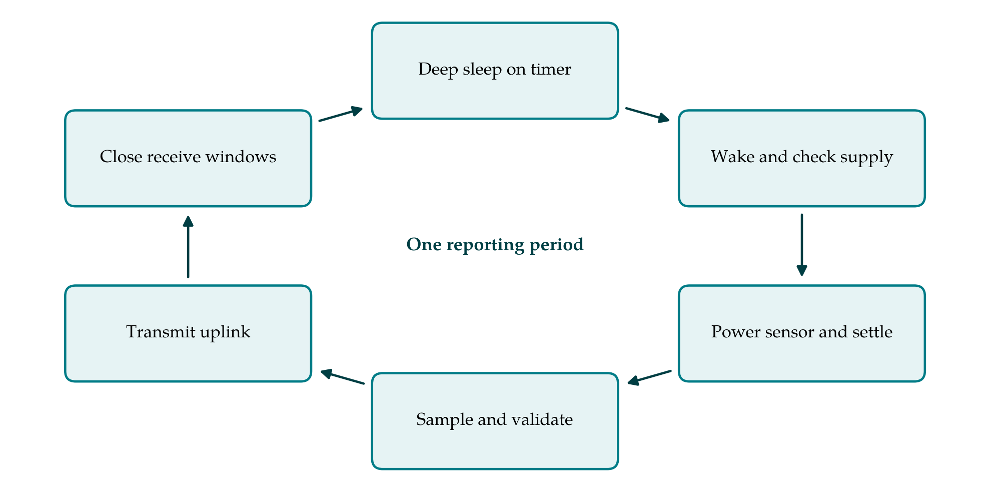
The probe should be powered through a switch controlled by the microcontroller and left off between readings. The firmware waits for the settling time the manufacturer specifies, takes several samples, and checks them for plausibility before accepting a value. Readings outside the physical range, or inconsistent within a burst, are flagged and not transmitted as data. Supply voltage is recorded with each reading, both because some probes are ratiometric and because it is the main health indicator available. Figure 1 shows the resulting sequence of states in one reporting period.
3.5. Step 5: Set the radio policy
With a class A LoRaWAN radio the energy per report is set by time on air. The payload should be a compact binary record, and several readings can be carried in one uplink where latency allows. Adaptive data rate lets the network move a node with a good link to a faster rate; a node at the edge of coverage will sit at the slowest rate, and the budget must be computed for that case if such nodes are expected. Confirmed uplinks and retries are costly and should be limited to messages that justify them. A cap on retransmissions protects the battery when a gateway is down.
3.6. Step 6: Eliminate sleep-state leakage
Sleep current is examined component by component. A regulator chosen for convenience may have a quiescent current larger than the rest of the sleeping node combined, and where the cell voltage suits the microcontroller and radio directly it can sometimes be removed. Pull-up resistors on lines that idle low, floating inputs, level shifters, indicator lamps and debug interfaces are all common drains. The microcontroller should be placed in its deepest mode that retains a timer, with unused peripherals and their clocks disabled, and the radio must be commanded to sleep explicitly after the receive windows close.
3.7. Step 7: Harden the hardware for the field
Electrical design counts for little if water reaches the board. The enclosure should carry an ingress protection rating suited to burial or exposure (IEC, 2013), cable entries should be glanded and sealed, and a conformal coating on the board limits the leakage currents that condensation causes. A pressure-equalising vent reduces the pumping of moist air through seals as temperature cycles. A capacitor of suitable size across a bobbin-type cell supplies the transmit pulse and masks the passivation delay. Connectors, the antenna and the probe cable should be chosen with rodents, ultraviolet light and farm machinery in mind, since published deployment reports attribute many lost nodes to mundane physical causes of this kind (Barrenetxea et al., 2008).
3.8. Step 8: Verify and plan for monitoring
The redesigned node is profiled with an instrument able to resolve both sleep current and transmit peaks, over many complete cycles and at the temperature extremes of the mission profile. The measured daily charge is compared with the budget from step 3. Verification does not end at deployment. Each uplink should carry supply voltage under load, a reset counter and the count of failed transmissions, so that an abnormal drain shows in the data long before the cell is exhausted.
4. Fitting the Procedure to Practice
The steps are ordered so that cheap decisions come before expensive ones. Steps 1 to 3 need only a spreadsheet and a bench measurement, and they often show that one or two states account for most of the charge. Firmware changes in steps 4 and 5 can be made on existing hardware. Steps 6 and 7 usually mean a board revision and a new enclosure, and are best done together. A team with a deployed fleet may apply the firmware steps first and reserve the hardware steps for the next production run. Where the audit shows that the budget cannot be met at the required reporting interval, the mission profile is revisited before any component is changed.
5. Limitations and What Remains to Be Shown
The procedure rests on published experience and on reasoning, and it carries the limits of both. A current budget predicts battery life only as well as its derating factors, and the behaviour of lithium thionyl chloride cells over years of pulsed, low-rate discharge at varying temperature is hard to predict from short tests. Bench profiling cannot reproduce five years of weather. Sensor drift and the loosening of soil contact around a probe are outside the energy analysis altogether and may limit useful life before the battery does. A proper validation would apply the procedure to a real node, record the audit and the budget, deploy a group of redesigned nodes beside unmodified ones, and follow their telemetry for long enough to compare predicted and observed drain. Until that is done the procedure should be read as a structured checklist with reasons attached.
6. Conclusion
A five-year soil moisture node is within reach of ordinary components if the design is approached as an accounting exercise. The proposed procedure fixes the mission, measures where the charge goes, sets a budget the battery can honestly meet, and then works through sensing, radio, sleep state and physical protection in turn before checking the outcome against the budget. Its merit, if field use bears it out, would lie in making the assumptions explicit at each step, so that when a deployed node falls short the reason can be traced.
Conflict of interest
To be declared by the author(s) before publication.
Funding
To be declared by the author(s) before publication.