1. Introduction
A wireless sensor network is a collection of small devices that measure something, a temperature, a vibration level, a pollutant concentration, and pass their readings to one another by short-range radio (Akyildiz et al., 2002). The readings are correlated, because neighbouring sensors observe nearly the same physical field, and that correlation is what makes compression, denoising and interpolation possible. On a regular grid the tools for exploiting it are a century old. On the scattered layouts that deployments produce, with sensors clustered along corridors and sparse elsewhere, Fourier analysis and uniform sampling theory do not apply directly.
Graph signal processing offers a replacement. It represents the network as a graph whose vertices are the sensors and whose weighted edges express similarity or connectivity, and it treats one snapshot of readings as a function on the vertices. Two overlapping formulations appeared in close succession. One builds on spectral graph theory and the graph Laplacian (Shuman et al., 2013). The other starts from the adjacency matrix as a shift operator and extends the algebra of discrete-time systems (Sandryhaila and Moura, 2013). The overview by Ortega et al. (2018) reconciles them and surveys applications.
Sensor networks were among the motivating examples in all of these papers, and they remain a good test of the theory because their constraints are strict: little energy, limited bandwidth, unreliable links and no central clock. This review asks what graph signal processing currently provides under those constraints, concentrating on filtering and sampling.
2. Approach of the Review
This is a narrative review of the published literature. It is organised by concept, not by chronology, and relies on the tutorial and overview articles of the field together with the papers that introduced each main technique. The selection favours results that bear on sensor networks with fixed node positions and scalar measurements. Graph neural networks, which grew out of the same filtering ideas, are mentioned only where they touch the subject, since their training requirements place them outside the resource budget of most sensor nodes. Mathematical statements are given in words or in simple inline form.
3. From Sensor Layout to Graph Signal
Everything in graph signal processing depends on a matrix that describes the graph. For an undirected graph with a symmetric weight matrix W, the combinatorial Laplacian is L = D - W, where D is the diagonal matrix of vertex degrees. L is symmetric and positive semidefinite, so it has real non-negative eigenvalues and an orthonormal set of eigenvectors (Chung, 1997). The quadratic form of a signal x with L equals the weighted sum of squared differences across all edges, and it is small exactly when strongly connected vertices carry similar values. The eigenvectors, ordered by eigenvalue, therefore run from smooth to oscillatory, and the eigenvalues play the part of frequencies.
The graph Fourier transform of a signal is its expansion in this eigenvector basis. A signal whose expansion uses only the eigenvectors of the lowest eigenvalues is called bandlimited, by analogy with the classical case. In the adjacency-based formulation the eigenvectors of the shift matrix serve the same purpose, and frequency is ordered by how much a signal changes under one application of the shift (Sandryhaila and Moura, 2014). For undirected graphs the two views give closely related results. They part company on directed graphs, a point taken up among the open problems below.
3.1. Constructing the graph
A sensor network comes with at least two candidate graphs. The communication graph joins nodes that can exchange packets. A similarity graph joins nodes whose readings are expected to be alike, most often through a Gaussian kernel of the distance between them, restricted to the nearest neighbours or to pairs closer than a threshold, a construction familiar from manifold learning (Belkin and Niyogi, 2003). The two need not coincide: sensors on opposite sides of a wall may hear each other well and measure quite different temperatures.
When past readings are available, the graph can be estimated from them. One line of work looks for the Laplacian under which the observed signals are smooth (Dong et al., 2016). Another assumes the signals are outputs of a diffusion on the unknown graph and recovers its eigenvectors from the sample covariance. The surveys by Mateos et al. (2019) and Dong et al. (2019) organise this literature. For a sensor network the practical tension is that a learned graph may contain edges between nodes that are out of radio range, and a filter defined on such a graph can no longer be run by neighbour-to-neighbour exchange.
4. Graph Filters
A graph filter modifies the graph Fourier coefficients of a signal, attenuating some frequencies and keeping others. Applied literally, this needs the full eigendecomposition and a central processor. The value of the theory for sensor networks lies in filters that avoid both.
4.1. Polynomial filters and distributed implementation
A polynomial in the Laplacian or the adjacency matrix is a graph filter whose frequency response is the same polynomial evaluated at the eigenvalues. Multiplying a signal by the matrix once requires each node only to combine its own value with those of its neighbours, so a polynomial of degree K is computed in K rounds of local exchange, and its output at a node depends only on nodes within K hops. This is the graph counterpart of a finite impulse response filter. Hammond et al. (2011) used Chebyshev polynomial approximation to realise arbitrary smooth responses without an eigendecomposition, and Shuman et al. (2018) developed the same idea into a distributed processing scheme for networks, with an account of the communication cost. Design methods that fit the polynomial coefficients to a desired linear operator are given by Segarra et al. (2017).
Polynomial filters have a familiar weakness. A sharp transition between passband and stopband needs a high degree, and each extra degree is another round of radio transmissions from every node. The coefficients also depend on the spectrum of the particular graph, so that a filter designed for one topology has to be redesigned when links change.
4.2. Rational filters
Rational responses, the graph analogue of infinite impulse response filters, obtain sharper transitions with fewer parameters. Isufi et al. (2017) proposed autoregressive moving average graph filters that are computed by a local recursion, each node repeatedly mixing its previous output with its neighbours' outputs and the input, and that converge to the desired response. Because the recursion keeps running, such filters follow slow changes in the signal and tolerate some variation in the graph, which suits a network whose links fade in and out. Convergence imposes conditions on the coefficients, and the number of iterations needed for a given accuracy is the quantity to weigh against the degree of an equivalent polynomial filter.
4.3. Wavelets and filter banks
Smoothing is one use of filtering. Another is multiscale analysis, which separates a sensor field into coarse trends and local detail and is the basis of transform coding. Spectral graph wavelets are obtained by dilating a band-pass kernel in the graph frequency domain and are localised around each vertex (Hammond et al., 2011). They form an overcomplete representation. Critically sampled alternatives were constructed by Narang and Ortega (2012) as two-channel filter banks with perfect reconstruction on bipartite graphs, with general graphs handled by decomposition into bipartite subgraphs. For data gathering, a critically sampled transform means no more coefficients are transmitted than there are sensors. Table 1 sets the main filter types side by side.
| Filter class | How it is computed | Strength | Limitation |
|---|---|---|---|
| Spectral (exact) | Full eigendecomposition at a central node | Any frequency response | Cost grows quickly with network size |
| Polynomial (FIR) | K rounds of exchange between neighbours | Strictly local; simple | High degree for sharp responses |
| Rational (ARMA) | Local recursion run to convergence | Sharp response with few coefficients | Stability and convergence conditions |
| Spectral wavelets | Bank of polynomial filters at several scales | Localised multiscale analysis | Overcomplete output |
| Two-channel filter bank | Filtering plus downsampling on bipartite graphs | Critically sampled | Requires bipartite decomposition |
5. Sampling and Reconstruction
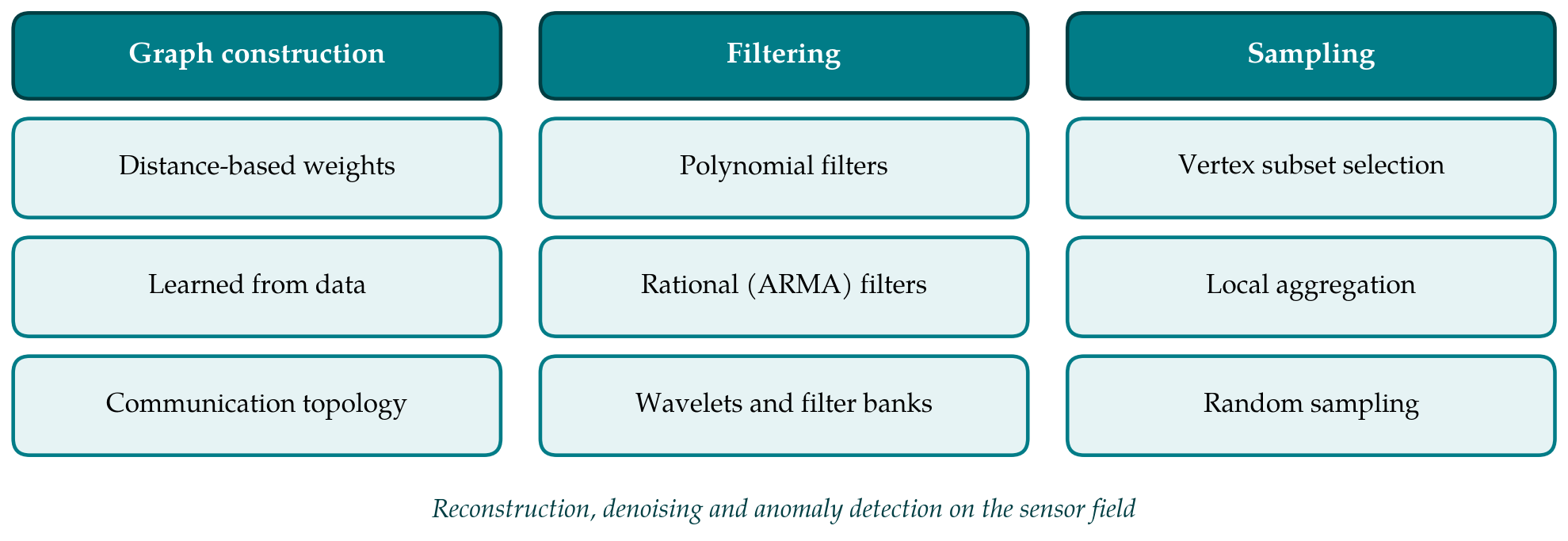
Sampling theory on graphs asks when a signal can be recovered from its values on a subset of the vertices. For a sensor network the subset has two readings. It may be the set of locations at which sensors are installed at all, or the set of installed sensors that are awake and reporting in a given round while the others sleep to save energy. Figure 1 places sampling beside graph construction and filtering as the three components from which applications are assembled.
5.1. Conditions for recovery
Pesenson (2008) established that signals whose graph Fourier coefficients vanish above a cut-off are determined by their values on suitable vertex subsets, which he called uniqueness sets. Later work turned this into linear algebra. If a signal lies in the span of K known eigenvectors, it can be recovered from the samples on a vertex set exactly when the rows of the eigenvector matrix belonging to that set have rank K, and recovery is then a least-squares problem (Chen et al., 2015). At least K samples are needed, and for almost every graph some set of exactly K suffices. Tsitsvero et al. (2016) connected the condition to an uncertainty principle that limits how concentrated a signal can be on a vertex set and a frequency set at once.
5.2. Choosing the sampling set
Not every valid sampling set is a good one. With noisy readings the reconstruction error depends on the conditioning of the sampled eigenvector matrix, and finding the best set is a combinatorial problem. Greedy selection, adding one vertex at a time to improve a criterion borrowed from experimental design, is the common answer. The difficulty for large networks is that the criteria need the eigenvectors. Anis et al. (2016) avoided the decomposition with spectral proxies, powers of the Laplacian that estimate the bandwidth a candidate set can support. Puy et al. (2018) took a probabilistic route, drawing vertices at random from a distribution adapted to the graph and proving stable recovery when the number of samples is of the order of K log K.
5.3. Aggregation sampling and reconstruction in the network
A different scheme observes one node repeatedly instead of many nodes once. Marques et al. (2016) showed that a bandlimited signal can be recovered from successive applications of the shift operator observed at a single vertex, that is, from what one node sees as its neighbours' values diffuse towards it. For sensor networks this trades wide-area communication for local iterations. Reconstruction from samples can likewise be written as an iteration of local operations, so that sleeping nodes have their values interpolated by their neighbours without a fusion centre. The review by Tanaka et al. (2020) sets out these variants and notes that the bandlimited model itself is an assumption; smoothness priors and piecewise-smooth models lead to different sampling rules.
6. Open Problems
Directed graphs come first. Sensor links are often asymmetric, and physical fields with advection, such as a pollutant carried by wind, are better described by a directed graph. The Laplacian framework assumes symmetry. The adjacency framework accepts directed graphs but may meet a shift matrix that is not diagonalisable, in which case the Fourier basis is defined through the Jordan decomposition and is numerically fragile (Sandryhaila and Moura, 2014). Several alternative definitions have been proposed, and no single one has been accepted as standard.
Uncertainty in the graph is the second problem. Edge weights are set by a kernel width chosen by hand or estimated from limited data, and links fail. Filters and sampling sets designed for a nominal graph are then applied to a different one. Stability results exist for particular filter classes, and the question has been studied closely in the context of graph neural networks (Gama et al., 2020), but a general account of how errors in the graph propagate to errors in reconstruction is missing. A related gap is the lack of a principled way to choose among several plausible graphs for the same deployment.
Third, sensor data are time series, and the graph may change while they are collected. Joint time-vertex methods treat the data as a signal on the product of a path graph for time and the sensor graph (Grassi et al., 2018), and the notion of stationarity has been extended to graphs to support Wiener-type estimation (Perraudin and Vandergheynst, 2017). Both assume a fixed topology. Networks with mobile nodes or duty-cycled links need a theory in which the shift operator varies with time.
The last problem is the distance between the models and the hardware. Analyses usually count rounds of exchange and assume synchronous, lossless, real-valued communication. Deployed nodes quantise, lose packets, drift in time and pay for every transmission in battery life. Work on filtering with quantised or asynchronous exchanges has begun, yet few studies evaluate a complete chain of graph construction, filtering and sampling against a conventional baseline under a stated energy budget. Until that is done routinely, it will remain unclear how much of the theoretical gain survives in deployment.
7. Conclusion
Graph signal processing gives irregular sensor networks what uniform sampling theory gave regular arrays: a definition of frequency, a family of filters that can be computed where the data are, and conditions under which a subset of measurements determines the rest. Polynomial and rational filters make denoising a matter of neighbour exchanges, and sampling theory turns sensor selection and sleep scheduling into problems with clear criteria. The unresolved questions concern the foundations as much as the engineering. They include which graph to use, what frequency means when links are directed, and how the methods behave when the graph is wrong or moving. Answers to these will decide whether the framework becomes routine practice in sensor network design.
Conflict of interest
To be declared by the author(s) before publication.
Funding
To be declared by the author(s) before publication.