1. Introduction
Structure-based design is part of the standard curriculum in pharmaceutical science, and students are expected to leave with some feeling for what a docking score does and does not mean. Delivering that in a laboratory session is harder than it looks. Commercial suites are expensive per seat and are usually installed only on the machines of research groups. Public web servers run a calculation for the student and return a picture, which teaches the vocabulary but not the craft: the student never chooses a protonation state, never defines a search box, never notices that a crystallographic water was in the way.
The alternative is to assemble the laboratory from open source components. The pieces have been available for some years and are well documented. AutoDock Vina performs rigid-receptor docking quickly enough for a class (Trott and Olson, 2010; Eberhardt et al., 2021). RDKit handles the cheminformatics (Landrum, 2023) and Open Babel the file conversions (O'Boyle et al., 2011). GROMACS runs molecular dynamics at a speed that makes a short alchemical calculation feasible on a workstation with a consumer graphics card (Abraham et al., 2015), and the Open Force Field initiative supplies small-molecule parameters without a licensed typing program (Qiu et al., 2021).
What has been missing is not software but a sequence: an order of steps, with the checks that make the output meaningful, that fits two or three timetabled sessions and can be marked. This article proposes such a workflow. It is offered as a design and has not been validated with students here.
2. Background and Design Considerations
Three constraints shaped the design. The first is the honesty of the exercise. Docking programs reproduce crystallographic binding modes reasonably often but rank affinities poorly, a limitation documented since the comparative evaluations of Warren et al. (2006) and discussed for the practitioner by Kitchen et al. (2004). A teaching laboratory that presents a docking score as a predicted affinity teaches something false. The workflow therefore pairs docking with a physically grounded method on a small scale, so that students see both the convenience of the fast approach and the cost of the accurate one.
The second constraint is time. Relative binding free energy calculations of the kind described by Wang et al. (2015) need many windows per perturbation and substantial hardware. Restricting the class to a single pair of closely related ligands, with short sampling and a prepared starting configuration, brings one perturbation within a session while preserving the concepts: the thermodynamic cycle, the alchemical pathway, the need for overlap between neighbouring states, and the estimate of statistical error. The multistate Bennett acceptance ratio of Shirts and Chodera (2008) supplies the estimator and an uncertainty with it.
The third is reproducibility. Every step is driven by a short script under version control rather than by clicking, so that a demonstrator can repeat a student submission exactly. This also makes the laboratory portable between institutions, which matters because installation support is the usual reason such courses are abandoned.
3. The Proposed Workflow
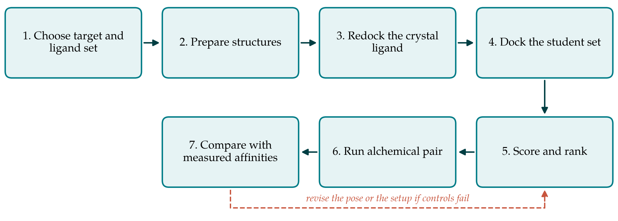
The workflow has seven steps. Table 1 lists them with the tool used, the judgement the student exercises and the artefact to be submitted. Figure 1 shows how the steps connect and where the exercise loops back when a control fails. Each step is then described in turn.
| Step | Open source tool | Judgement required of the student | Artefact submitted |
|---|---|---|---|
| 1. Choose system | RDKit, PDB entry | Is the structure good enough and the ligand series congeneric | Short justification note |
| 2. Prepare structures | PDBFixer, Open Babel | Protonation, tautomers, which waters to keep | Prepared receptor and ligand files |
| 3. Redock control ligand | AutoDock Vina | Box placement and exhaustiveness setting | Deviation from the crystal pose |
| 4. Dock the set | AutoDock Vina | Whether each pose is chemically sensible | Pose file and annotated figure |
| 5. Score and rank | RDKit, Python | How far the ranking should be trusted | Ranked table with commentary |
| 6. Alchemical pair | GROMACS, Open Force Field | Window spacing and length of sampling | Free energy difference with error |
| 7. Compare and report | Python plotting | Which disagreements matter and why | Laboratory report |
3.1. Step 1: Choose the target and the ligand set
The target should have a crystal structure at good resolution with a bound ligand of reasonable quality, a buried rather than shallow site, and a published series of analogues with measured affinities spanning at least two orders of magnitude. Kinases, serine proteases and carbonic anhydrases are dependable choices. The demonstrator supplies two or three candidate systems rather than leaving the search open, since finding a suitable system is a research skill of its own and consumes a whole session. Students write a paragraph justifying the choice, which obliges them to look at the electron density fit of the ligand and the presence of crystallisation additives in the site.
3.2. Step 2: Prepare the structures
Preparation is where most of the learning sits. The receptor is cleaned with PDBFixer: alternate conformations resolved, missing side chains rebuilt, hydrogens added at the chosen pH. The student decides which crystallographic waters to retain, which forces an argument about whether a water is a structural part of the site or a solvent molecule in the way. Ligands are drawn or imported as SMILES, protonated at physiological pH, and converted to three-dimensional conformers with RDKit, whose conformer generation follows the distance geometry approach refined by Riniker and Landrum (2015). Open Babel handles conversion to the format Vina expects. The common failure here is a ligand charge state assigned by default rather than by thought, and the demonstrator should ask each student to defend the protonation of any ionisable group.
3.3. Step 3: Redock the crystallographic ligand
Before any new compound is docked, the student removes the crystal ligand, docks it back, and measures the root mean square deviation of the best-scoring pose from the deposited coordinates. This is the control. If the deviation is large the setup is wrong, and the usual causes are a search box that is too small or wrongly centred, a missing metal ion or cofactor, or a water that should have been kept. The exercise should not proceed until the control passes, and the loop shown in Figure 1 exists for this purpose. Students who pass the control on the first attempt are asked to repeat it with a deliberately undersized box so that they see the failure mode.
3.4. Step 4: Dock the student set
The prepared analogues are docked with the settings validated in step 3, with the exhaustiveness setting raised and several independent runs per ligand so that the reproducibility of the search can be inspected. Each student examines the top poses by eye in a molecular viewer and asks whether the interactions are chemically reasonable: hydrogen bonds with sensible geometry, hydrophobic groups buried, no charged group left pointing into the lipophilic wall of the site. Poses that score well and look wrong are the most instructive output of the session, and students are asked to keep one.
3.5. Step 5: Score, rank and interpret
Scores are collected into a table and plotted against the measured affinities taken from the literature source for the series. Agreement is usually poor, and the discussion that follows is the point of the step. Students are asked to say which ligands are ranked badly and to propose explanations: unmodelled receptor flexibility, a desolvation cost the function treats crudely, a ligand strain not accounted for, or an experimental affinity measured under different conditions. The limitations reported by Warren et al. (2006) give them a vocabulary for this, and the practical account of Vina given by Eberhardt et al. (2021) explains what the scoring function actually contains.
3.6. Step 6: One alchemical free energy calculation
A single pair of ligands differing by one small substituent is chosen, and the relative binding free energy is computed along an alchemical path in the complex and in water. Parameters come from an Open Force Field small-molecule force field (Qiu et al., 2021) with a standard protein force field and an explicit water model; GROMACS runs the windows (Abraham et al., 2015) and the estimate is obtained with the multistate Bennett acceptance ratio (Shirts and Chodera, 2008), which also reports an uncertainty. Soft-core potentials are used for the decoupling, following the treatment of Beutler et al. (1994), and the student inspects the overlap between neighbouring windows before trusting the number. To keep the step within a session the demonstrator supplies equilibrated starting configurations and a prepared input set, so that the student spends the time on the analysis rather than on system setup.
3.7. Step 7: Compare and report
The report brings the three sources together: the measured affinity difference for the pair, the difference implied by the docking scores, and the alchemical estimate with its error bar. Students are asked to state which method they would use to triage a virtual library of many compounds, which to compare two candidates before synthesis, and what the cost of each is in computer time. A good report will note that the alchemical result can be precise and still inaccurate if the force field or the binding mode is wrong, and that both methods inherit whatever error was made during preparation.
4. Fitting the Workflow to a Teaching Programme
The workflow is designed for three sessions of about three hours: preparation and the redocking control; docking of the set with scoring and interpretation; the alchemical pair with the comparison and report. Hardware is modest. Docking runs comfortably on laptops, while the free energy step needs a shared workstation with a consumer graphics card, or a small allocation on an institutional cluster, and can be submitted at the end of the second session so that results are waiting at the start of the third. Installation is best handled with a prepared environment file or a container image, because dependency problems consume teaching time and discourage reuse.
Assessment follows the artefacts in Table 1. Marks are given for the quality of the justifications and for the handling of the control rather than for obtaining a particular answer, which keeps the incentive on the reasoning. A class with little programming experience can be given notebooks with the commands filled in and the parameters left blank. Students with more background can be asked to script the whole sequence and to run a small cross-docking exercise as an extension.
5. Limitations and What Remains to Be Shown
This article proposes a laboratory and does not evaluate it. Several things would need to be observed before it could be recommended without qualification. The first is timing: whether the steps as written actually fit the sessions, with a class of mixed ability and shared hardware. The second is attainment: whether students who complete the workflow understand the limits of docking scores better than those taught with a web server, which would need a comparison with a suitable instrument. The third is robustness of the software stack across the machines a department actually owns, including the question of whether the free energy step completes reliably without specialist support.
Two cautions apply to the content itself. The alchemical step is reduced so far that it demonstrates a method rather than producing a result anyone should rely on, and this must be said plainly to students. And the whole workflow treats the receptor as rigid apart from the short dynamics in step 6, so systems with substantial induced fit should be avoided when the target is chosen.
6. Conclusion
A teaching laboratory in structure-based design can be assembled from freely available software and run on the hardware a department already owns. The seven-step workflow proposed here places a crystallographic redocking control before any student result is accepted, makes the weakness of docking scores an object of study rather than an embarrassment, and ends with a single alchemical calculation that shows what a more rigorous method costs. Whether it teaches better than the alternatives is an empirical question, and one that departments adopting it are well placed to answer.
Conflict of interest
To be declared by the author(s) before publication.
Funding
To be declared by the author(s) before publication.