1. Introduction
Oscillating foils have been studied for decades as models of the fins and wings of swimming and flying animals and as propulsors in their own right. Flow visualisation by Koochesfahani (1989) showed that the pattern of vortices shed by a pitching aerofoil can be switched between a drag-producing and a thrust-producing arrangement by changing frequency and amplitude. Triantafyllou et al. (1991) connected efficient thrust to a band of Strouhal number, and Anderson et al. (1998) related high propulsive efficiency to the timing of leading-edge vortex shedding. Cruising animals were later found to operate within a similar band, with Strouhal numbers between about 0.2 and 0.4 (Taylor et al., 2003).
Those results rest largely on two-dimensional pictures. A real foil has finite span, and its wake is three-dimensional from the start. von Ellenrieder et al. (2003) visualised the wake of a heaving and pitching wing as a set of linked vortex rings, and Buchholz and Smits (2008) showed for a low-aspect-ratio pitching panel that the wake compresses in the spanwise direction and can split into two oblique trains. Quantifying such structures requires velocity gradients in all three directions at once.
Tomographic particle image velocimetry (tomographic PIV), introduced by Elsinga et al. (2006), provides exactly that. This article sets out a workflow for using it behind a flapping foil. The workflow is a proposal built from the published literature; no measurements are reported, and the procedure has not been validated here.
2. Background: What the Technique Requires
In tomographic PIV a volume of seeded fluid is illuminated and viewed by several cameras from different directions. The three-dimensional distribution of particle intensity is reconstructed from the simultaneous images, usually with the multiplicative algebraic reconstruction technique (MART) of Herman and Lent (1976), and pairs of reconstructed volumes are cross-correlated to give displacement. Scarano (2013) reviews the principles and the accumulated experience. Three features dominate planning. Reconstruction quality falls as seeding density rises, because spurious intensity peaks known as ghost particles form where lines of sight from real particles intersect by chance. The mapping between image and physical space must be accurate to a small fraction of a pixel. And the laser energy is spread over a thick volume while the lenses are stopped down for depth of focus, so light is scarce. General practice for PIV recording and evaluation is covered by Raffel et al. (2018).
3. The Proposed Workflow
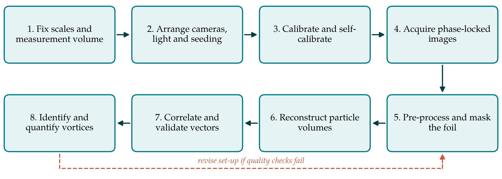
The workflow has eight steps, listed in Table 1 with the principal decision and the check attached to each. Figure 1 shows the sequence and the return path taken when a check fails. The subsections below take the steps in order, grouping those that are decided together.
| Step | Main decision | Quality check before proceeding |
|---|---|---|
| 1. Scales and volume | Volume size and position relative to the trailing edge | Volume spans at least one shedding wavelength |
| 2. Optics and seeding | Number of cameras, aperture, particle image density | Particles in focus through the depth; density near 0.05 per pixel |
| 3. Calibration | Target traverse and mapping function | Self-calibration residual below 0.1 pixel |
| 4. Acquisition | Phases sampled and repetitions per phase | Foil position recorded with every image pair |
| 5. Pre-processing | Background removal and foil mask | Uniform particle intensity; no foil reflections |
| 6. Reconstruction | Algorithm, iterations, voxel size | Intensity profile through depth shows clear volume edges |
| 7. Correlation | Interrogation volume and overlap | Few outliers; small residual divergence |
| 8. Vortex analysis | Identification criterion and threshold | Circulation consistent between neighbouring planes |
3.1. Steps 1 and 2: Scales, volume, optics and seeding
Planning starts from the flow and not from the equipment. The chord, the flapping frequency and the free-stream speed fix the Strouhal number and the streamwise spacing of the shed vortices; the trailing-edge excursion gives the initial wake width. The measurement volume should hold at least one full shedding wavelength in the stream direction and the whole span of the structures of interest, with the trailing edge either just inside the volume or just upstream of it. Where one volume cannot do both, overlapping volumes at successive downstream stations, each sampled at the same phases, are preferable to a single volume stretched too thin.
Volume thickness is the costly dimension, since light intensity falls and ghost intensity rises with it. Four cameras are the usual compromise. They are placed with a total angular aperture large enough to resolve depth, fitted with Scheimpflug adapters so that the focal plane lies along the mid-plane of the volume, and stopped down until particles remain in focus across the full thickness. For a four-camera system a particle image density of about 0.05 particles per pixel is the accepted working value (Elsinga et al., 2006; Scarano, 2013). The volume edges should be cut sharply with knife-edge slits, both to keep stray particles out of the lines of sight and to make the reconstructed depth profile a usable diagnostic later.
3.2. Step 3: Calibration
A target is traversed through the depth of the volume and a mapping function is fitted for each camera. This physical calibration is rarely accurate enough by itself, because small movements of the cameras, the tank walls or the target leave errors of a pixel or more. Volume self-calibration, introduced by Wieneke (2008), uses the particle images themselves: particles are triangulated, the residual disparity between cameras is mapped through the volume, and the mapping functions are corrected. Reducing the residual to below about 0.1 pixel is the accepted requirement for reconstruction. In a facility with a moving foil and carriage the self-calibration should be repeated whenever anything is disturbed and at intervals during a long campaign, using recordings at reduced seeding if necessary.
3.3. Steps 4 and 5: Acquisition, pre-processing and masking
Low-repetition tomographic systems cannot follow a flapping cycle in time, so acquisition is locked to the phase of the motion. An encoder on the actuator triggers the laser and cameras at chosen phases, and the measured foil position is stored with each image pair. The number of phases should resolve the formation and release of each vortex, and the number of repetitions at each phase should be set by the convergence of phase-averaged vorticity, which is slower than that of velocity. Where a time-resolved system is available, the same workflow applies and tracking-based methods such as Shake-The-Box (Schanz et al., 2016) become an alternative to correlation.
Phase averaging deserves a deliberate choice of reference. Averaging at fixed phase of the foil motion is the natural default and separates the periodic wake from the residual fluctuation. Further downstream, where vortices wander from cycle to cycle, a fixed-phase average smears their cores and understates peak vorticity. Keeping the instantaneous fields allows a conditional average, aligned on the detected position of each vortex, to be formed afterwards and compared with the fixed-phase result. The difference between the two is itself informative, since it measures how repeatable the wake is at that station.
The foil itself is the main nuisance in the images. It reflects laser light, blocks lines of sight differently for each camera and shadows part of the volume. Matt black or fluorescent coatings reduce reflections at source. In pre-processing, a sliding minimum over each phase removes the stationary background, intensity is normalised between cameras, and a mask derived from the known foil geometry and the recorded position is projected into every camera image. Voxels that fewer than three cameras can see should be flagged and excluded, since reconstruction there is unreliable.
3.4. Step 6: Reconstruction
MART with around five iterations is the reference choice (Elsinga et al., 2006). Faster schemes that begin from a multiplicative first guess and update all voxels simultaneously were introduced by Atkinson and Soria (2009) and are now standard for large volumes. Where pairs of exposures are available, motion-tracking enhancement (Novara et al., 2010) uses the fact that real particles move coherently between exposures whereas ghosts do not, and so permits higher seeding. The voxel size is matched to the pixel size in physical units. The check on this step is the profile of reconstructed intensity through the depth: it should be flat inside the illuminated slab and drop sharply outside, and the ratio of the two levels is a direct indicator of ghost intensity.
3.5. Step 7: Correlation and validation
Displacements are obtained by three-dimensional cross-correlation with iterative volume deformation, ending at an interrogation volume that contains several particles and overlaps its neighbours. Spurious vectors are detected with the normalised median test of Westerweel and Scarano (2005), extended to three dimensions. Two checks are particular to volumetric data. For an incompressible flow the measured divergence should vanish, so its spread is a measure of error in the velocity gradients. And ghost particles, which move with the average displacement of the particles that create them, bias gradients toward zero across the depth; a vortex core that looks weaker in the depth direction than in the others is a warning sign.
3.6. Step 8: Vortex identification and quantification
Vorticity magnitude alone does not separate vortices from shear layers, and the wake of a flapping foil contains both. The Q criterion and the λ2 criterion, both set out and compared by Jeong and Hussain (1995), are the usual choices, applied to phase-averaged fields with a threshold stated explicitly. From the identified structures the analysis extracts the quantities that connect to performance: the circulation of each loop, obtained by integrating vorticity over planes cut through it; the spacing and inclination of successive loops; and the momentum carried by the jet between them. Circulation computed on neighbouring planes through the same vortex tube should agree, which gives a final internal check. Pressure fields and loads can be derived from the velocity data by the methods reviewed by van Oudheusden (2013), given adequate temporal information.
4. Fitting the Workflow to a Facility
Three constraints will shape any implementation. Optical access is the first: water tunnels and towing tanks often permit viewing from one side only, which limits the angular aperture and may call for water-filled prisms to reduce astigmatism at the wall. The second is light. Larger tracer particles and a double-pass arrangement with a mirror raise the signal, and the volume thickness may need to be set by the available pulse energy. The third is time. A phase-locked campaign over many phases, several downstream stations and a range of Strouhal numbers produces a large body of images, and reconstruction dominates the computing cost. Running the full chain on a short pilot recording before the main campaign exposes most problems while they are still cheap to fix.
The record kept with the data matters as much as the data. For each run the file should hold the foil kinematics as measured, the calibration and self-calibration residuals, the particle image density, the reconstruction settings, the interrogation volume in physical units and as a fraction of the chord, and the thresholds used for outlier detection and vortex identification. With that record a reader can judge whether a reported vortex core is resolved or merely detected, and a later campaign in another facility can be set up to match.
5. Limitations and What Remains to Be Shown
The workflow has not been tested here. Before it is relied on, three things should be demonstrated. The first is accuracy in this flow class: reconstructing synthetic images generated from a simulated flapping-foil wake, with a masked moving body, would show how ghost particles and masking bias the measured circulation. The second is agreement with an independent measurement, for example planar stereoscopic PIV through the mid-span, or thrust from a load cell compared with the momentum flux of the measured wake. The third is the uncertainty of derived quantities, which can be propagated from the velocity field by the approach of Sciacchitano and Wieneke (2016).
Some limits are inherent. Spatial resolution is set by the interrogation volume and will smooth vortex cores in small-scale experiments. Phase averaging removes cycle-to-cycle variation, which matters once the wake becomes irregular further downstream. And the region nearest the foil, where the vortices form, is the hardest to illuminate and view and the most affected by masking.
6. Conclusion
Resolving the vortex loops behind a flapping foil is a natural task for tomographic PIV, provided the experiment is planned around the scales of the wake and each stage of processing is checked before the next begins. The eight-step workflow proposed here gathers established guidance on volume design, calibration, reconstruction and vector validation and adds the steps that a moving body requires: phase locking, masking and visibility checks. It also ties the final analysis to quantities, circulation, loop geometry and wake momentum, that bear on propulsive performance. Whether the workflow delivers the accuracy needed for those quantities is an open question that a synthetic test and a comparison with independent measurements would answer.
Conflict of interest
To be declared by the author(s) before publication.
Funding
To be declared by the author(s) before publication.