1. Introduction
A suburban distribution feeder was designed for power to flow one way. Voltage is set at the substation, falls along the line as load is supplied, and is corrected where necessary by line regulators and switched capacitors. Rooftop photovoltaic (PV) systems disturb this arrangement at the hours when generation is high and household load is low. Power then flows from the low-voltage network back towards the substation and the voltage at the far end rises instead of falling, an effect described for embedded generation in general by Masters (2002) and for residential PV in particular by Tonkoski et al. (2012).
The utility usually learns of the matter indirectly. Inverters disconnect on over-voltage and their owners complain of lost production; a regulator logs many more tap operations than it used to; a neighbour without PV reports flickering lights on days of broken cloud. Such symptoms have different causes and call for different remedies, and the published work on remedies is large (Katiraei and Agüero, 2011; Bollen and Hassan, 2011). This article does not add another. It proposes an ordered assessment procedure by which a utility with ordinary planning tools can decide which of the known remedies suits a given feeder. No application of the procedure to an actual feeder is reported.
2. Background
The procedure rests on three bodies of established knowledge: the mechanism of voltage change, the limits that define an unacceptable voltage, and the range of available countermeasures.
2.1. Why rooftop generation moves feeder voltage
To a first approximation the voltage change across a line section is proportional to PR + QX, where P and Q are the active and reactive power transferred and R and X are the resistance and reactance of the section (Kersting, 2017). Low-voltage cables and small overhead conductors have a high ratio of resistance to reactance, so active power dominates the result, and exporting PV raises the voltage almost in proportion to its output. Single-phase connection adds unbalance, since installations are seldom spread evenly across the phases. Passing cloud superimposes changes over seconds to minutes, to which electromechanical tap changers, with their intentional time delays, respond late and repeatedly (Walling et al., 2008).
2.2. Limits that define a problem
Whether a voltage is acceptable is decided by the standard in force. In Europe, EN 50160 requires that ten-minute mean values of the supply voltage remain within ±10% of nominal for 95% of each week (CENELEC, 2010). In North America, ANSI C84.1 defines a preferred Range A for service voltage of ±5% of nominal (NEMA, 2020). Measurement methods, including the aggregation intervals on which such limits are assessed, are laid down in IEC 61000-4-30 (IEC, 2015). Inverter behaviour is governed by interconnection rules; IEEE Std 1547-2018 requires distributed resources to be capable of voltage regulation by reactive power and, in its higher performance category, by active power (IEEE, 2018).
2.3. The available remedies
Remedies act either at the inverter or on the network. Reactive power absorption by the inverters, at a fixed power factor or according to a volt-var curve, has been analysed by Turitsyn et al. (2011) and Carvalho et al. (2008), and its use through standardised inverter functions is described by Smith et al. (2011). Active power curtailment governed by a volt-watt droop was proposed by Tonkoski et al. (2011). Network measures include revised regulator settings, distribution transformers with on-load tap changers, conductor reinforcement and storage. German experience, where the question arose early and at scale, indicates that inverter-based measures and regulated transformers can defer much conventional reinforcement (Stetz et al., 2013; von Appen et al., 2013). Table 1 summarises the options.
| Option | How it acts | Principal limitation |
|---|---|---|
| Volt-var control at inverters | Inverters absorb reactive power as voltage rises | Weak on resistive low-voltage circuits; raises feeder current and losses |
| Volt-watt curtailment | Inverters reduce active power above a voltage threshold | Lost energy falls unevenly on customers at the feeder end |
| Revised regulator and capacitor settings | Lower set-point, wider bandwidth or longer delay | Must still support voltage at peak load without PV |
| On-load tap-changing distribution transformer | Decouples low-voltage level from medium-voltage level | Capital cost per transformer; no help with unbalance |
| Phase rebalancing | Moves single-phase connections between phases | Field work; benefit depends on existing unbalance |
| Reinforcement or reconfiguration | Lowers impedance between PV and source | Highest cost and longest lead time |
| Battery storage | Absorbs midday surplus and smooths ramps | Cost; needs a control scheme and an owner |
3. The Proposed Procedure
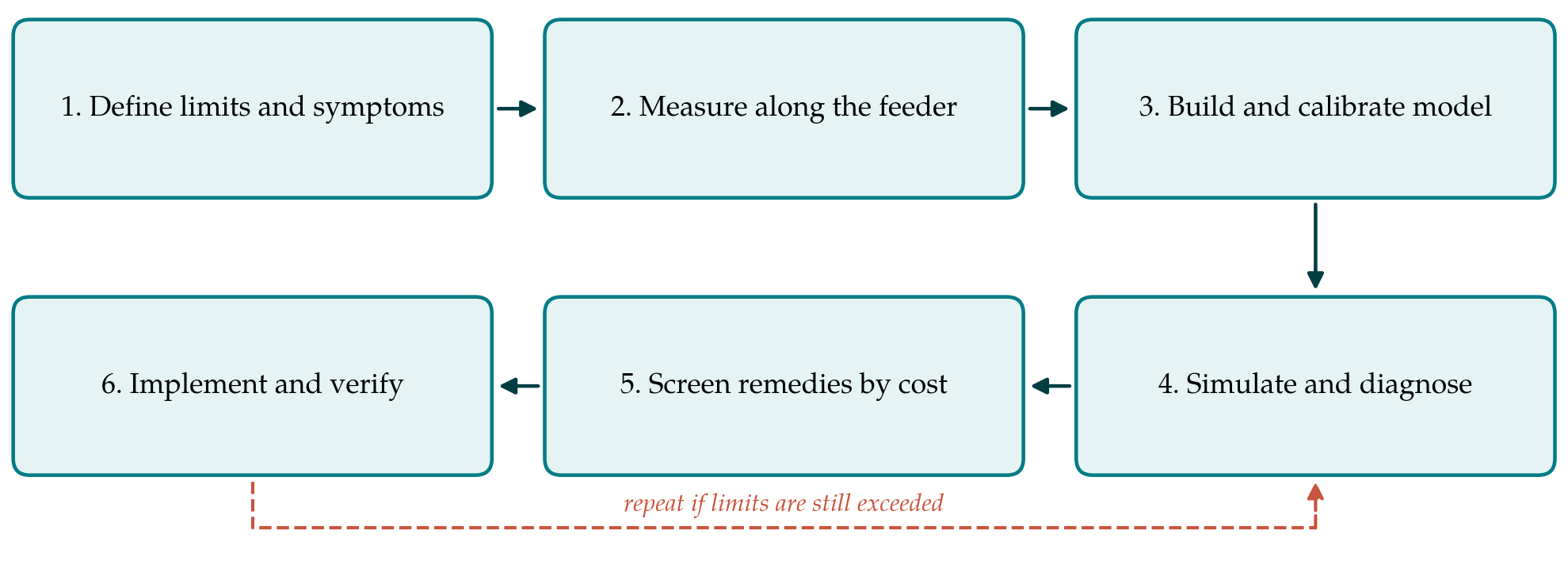
The procedure has six steps, shown in Figure 1. It is deliberately conservative: nothing is changed on the network until the cause has been located by measurement and reproduced in a model, and cheaper measures are examined before dearer ones.
3.1. Step 1: Define the limits and the symptoms
The engineer first records which standard and which interconnection rules apply, and therefore which quantity must stay within which band over which averaging interval. The reported symptoms are then sorted into three classes: sustained over-voltage at times of high generation, rapid fluctuation on partly cloudy days, and excessive operation of regulating equipment. Complaint records, inverter trip logs supplied by customers and the operation counters of regulators and capacitor controllers are the sources. The sorting matters because the first class is a steady-state problem, the second a dynamic one, and the third may be an artefact of control settings.
3.2. Step 2: Measure along the feeder
Measurement precedes modelling. Recorders complying with IEC 61000-4-30 are placed at the substation bus, at each regulator and at a small number of low-voltage points chosen to include the electrically most remote customers and the transformers with the highest PV capacity. Voltage per phase and active and reactive power are logged for a period long enough to contain clear days, overcast days and days of broken cloud at light load. Where smart meters report voltage, their data extend the coverage at no cost. If flicker is among the complaints, short-term flicker severity is recorded as well (Dugan et al., 2012).
3.3. Step 3: Build and calibrate a feeder model
A three-phase unbalanced model of the medium-voltage feeder is assembled from the utility's asset records, with the low-voltage networks of the affected transformers represented explicitly and the remainder lumped. Open-source tools such as OpenDSS are adequate for the purpose (Dugan and McDermott, 2011). The model is then run with the measured substation voltage and measured or estimated load and PV profiles, and its voltages are compared with the recordings from Step 2. Discrepancies usually trace to wrong phase assignments, wrong conductor data or incorrect regulator settings, and they are corrected in the model and, where relevant, in the asset records. The model is not used for decisions until it reproduces the measured voltage profile on both a high-generation and a high-load day.
3.4. Step 4: Simulate and diagnose
With a calibrated model, quasi-static time-series simulation over representative days answers three questions. Where and for how long does the voltage exceed the limit, and on which phase. How much of the excursion is slow rise attributable to reverse power flow and how much is fast variation with irradiance. And how do the regulators and capacitor banks respond, in particular whether they are operating against one another or against the inverters. The output of this step is a short written diagnosis that assigns each symptom from Step 1 to a cause and a location.
3.5. Step 5: Screen remedies in ascending order of cost
The options in Table 1 are tested in the model roughly in the order listed, stopping at the first that restores compliance with adequate margin at both light and peak load. Settings come first: inverter volt-var and volt-watt functions where the interconnection rules allow the utility to require them, then regulator set-points, bandwidths and time delays. Phase rebalancing is tried where the diagnosis shows marked unbalance. Capital measures follow. For each candidate the engineer records the residual violations, the change in losses and tap operations, the energy curtailed and who bears it, and an estimate of cost. Combinations are considered only when no single measure suffices.
3.6. Step 6: Implement and verify
The chosen measure is implemented and the measurements of Step 2 are repeated at the same points for a comparable period. Verification is by measurement, not by the model. If limits are still exceeded, the model is revised in the light of the new data and the procedure returns to Step 4. The file for the feeder should finally contain the diagnosis, the options examined with reasons for rejection, the settings applied and the before-and-after recordings, so that the next engineer to face additional PV on the same feeder starts from a calibrated model.
4. Fitting the Procedure to a Utility of Modest Means
Three practical points bear on adoption. Much of the cost lies in the first feeder, when recorders are bought and the modelling workflow is set up; subsequent feeders reuse both. Second, asset data are rarely as good as the model needs, and the calibration in Step 3 doubles as a data-quality exercise whose value extends beyond the voltage question. Third, inverter-based remedies depend on what the utility is entitled to ask of customers. Where legacy inverters lack the functions or the rules do not provide for them, the screening in Step 5 simply begins with network settings.
Fairness deserves explicit attention when curtailment is considered. A volt-watt function acts hardest on the installations at the end of the feeder, where the voltage is highest, so the owners there lose more energy than those near the transformer for the benefit of all. The literature has proposed coordinated schemes that share the reduction more evenly (Tonkoski et al., 2011); whether such a scheme is warranted is a policy question that the procedure makes visible but does not settle.
5. Limitations and What Remains to Be Shown
The procedure is a proposal built from standards and published methods, and it has not been validated here. Its usefulness would have to be shown by applying it to feeders with differing topology and PV density and recording whether the diagnosis from Step 4 was borne out by the verification in Step 6, how much effort each step consumed, and how often the cheapest adequate remedy turned out to be a change of settings. The procedure also inherits the limits of quasi-static simulation: it does not represent inverter control dynamics or harmonic interaction, and it addresses flicker only through measurement. It treats one feeder at a time and does not replace a hosting-capacity study of the whole network. Finally, it is reactive by design, starting from a symptom, and a utility expecting rapid PV growth would do better to run Steps 3 to 5 in advance.
6. Conclusion
Voltage problems after rooftop solar expansion are well explained and the remedies are known. The difficulty for a small utility is choosing among them with confidence. The six-step procedure proposed in this article orders the work as definition, measurement, calibrated modelling, diagnosis, cost-ordered screening and verification, and it asks at each step for a record that makes the decision traceable. It awaits trial on real feeders, and reports of such trials, including those in which it proved cumbersome or mistaken, would show where it needs to be changed.
Conflict of interest
To be declared by the author(s) before publication.
Funding
To be declared by the author(s) before publication.