1. Introduction
Shape analysis asks when two geometric objects should be regarded as similar and how that similarity can be measured from sampled data. Classical descriptors are geometric: curvature histograms, spectral signatures, distributions of pairwise distances. Topological descriptors answer a coarser question, how many pieces, loops and cavities a shape has, and for a long time they were considered too fragile for data, since a single stray sample or a small handle changes the Betti numbers.
Persistent homology repaired that fragility by replacing a single space with a nested family. As a threshold increases, features are born and die, and the length of the interval between the two events measures how prominent a feature is. The algorithm and the term persistence were introduced by Edelsbrunner et al. (2002), and the algebraic framing as a module over a polynomial ring, which explains why a barcode exists and extends the computation to arbitrary fields, is due to Zomorodian and Carlsson (2005). The expository articles of Ghrist (2008) and Carlsson (2009) brought the subject to a wide audience, and the textbook of Edelsbrunner and Harer (2010) remains the standard reference.
This review is organized around three questions that a practitioner of shape analysis has to face. How is persistence computed, and at what cost? In what sense is the output reliable when the input is noisy or sampled? And which computations remain out of reach? The intention is to connect results that are usually presented in separate literatures, algorithmic, algebraic and statistical, and to be explicit about the limits.
2. Scope and Approach
The article is a narrative review of the published literature, selective by design. It draws on the foundational papers, on a small number of surveys and monographs, and on the work that introduced each algorithmic idea discussed. Applications in particular sciences are mentioned only where they motivated a method. Software is discussed through the ideas it implements, and readers who need a comparison of packages are referred to the benchmark study of Otter et al. (2017). No claim of completeness is made, and extended variants such as zigzag and extended persistence are left aside.
3. From Shapes to Filtrations
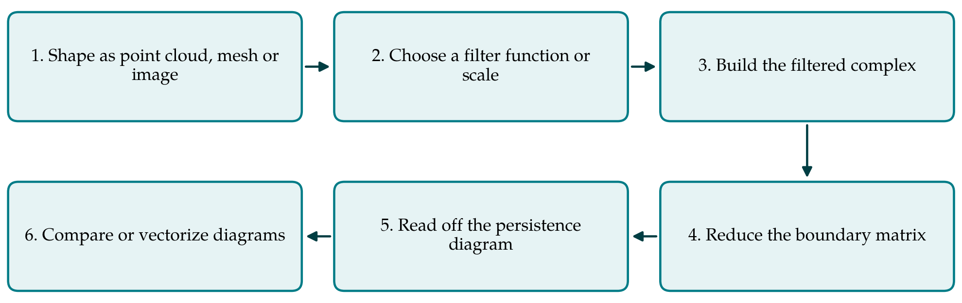
Every persistence computation follows the pipeline shown in Figure 1. A shape arrives as a point cloud, a triangle mesh or a voxel image. A filtration is then chosen, a complex is built, a matrix is reduced, and a diagram is produced and compared with others. The choices made at the second and third steps decide both what the diagram means and how large the computation becomes.
For point clouds the filtration is indexed by scale. The Čech complex at radius r is the nerve of the balls of radius r around the points and has the homotopy type of their union, but it is costly to construct. The Vietoris-Rips complex contains a simplex whenever all its vertices are pairwise within the threshold distance. It is determined by the distance matrix alone, which makes it the default for abstract metric data. The alpha complex, a subcomplex of the Delaunay triangulation introduced with alpha shapes by Edelsbrunner and Mücke (1994), carries the same homotopy type as the union of balls with far fewer simplices, and is the natural choice for shapes in the plane or in space. Witness complexes reduce size by building on a subset of landmark points (de Silva and Carlsson, 2004).
For meshes and images the filtration usually comes from a function. Sublevel sets of a height function, a geodesic distance, an eccentricity or a curvature measure give diagrams that describe the shape as seen through that function. Carlsson et al. (2005) proposed barcodes of derived spaces that encode tangential information as shape descriptors, and the persistent homology transform of Turner et al. (2014) collects the height-function diagrams over all directions and is injective for shapes in two and three dimensions, so that in principle no information is lost. Images are handled with cubical complexes, in which voxels play the part of simplices.
4. Algorithms
The standard algorithm orders the simplices by their time of entry, writes the boundary operator as a matrix in that order, and reduces it by left-to-right column additions until the lowest nonzero entries of the nonzero columns lie in distinct rows. Each such lowest entry pairs the simplex that creates a class with the one that destroys it. The reduction is a variant of Gaussian elimination and takes time cubic in the number of simplices in the worst case, although on the complexes met in practice it behaves far better (Edelsbrunner and Harer, 2010).
Three ideas account for most of the practical speed gained since. The first is clearing: a simplex already identified as destroying a class cannot create one, so its column can be set to zero without reduction, provided dimensions are processed in decreasing order (Chen and Kerber, 2011). The second is to compute persistent cohomology instead of homology. The barcodes are the same, but the coboundary matrix of a Vietoris-Rips filtration reduces much faster, and clearing then removes most of the remaining work (de Silva et al., 2011).
The third idea is never to store the matrix. Ripser enumerates cofaces on demand from the distance matrix, represents simplices by their index in a combinatorial number system, and recognizes many persistence pairs of zero length directly without reducing any column (Bauer, 2021). Together with clearing and cohomology this reduced both running time and memory by large factors compared with earlier codes, and its design has been adopted widely. The comparison by Otter et al. (2017) documents how strongly performance depends on the type of complex and on these implementation choices.
5. Stability Results
A descriptor is useful only if small changes in the input cause small changes in the output. For persistence the basic statement is the stability theorem of Cohen-Steiner et al. (2007): for two tame functions on a triangulable space, the bottleneck distance between their diagrams is at most the supremum norm of their difference. The bottleneck distance matches the points of two diagrams, allowing unmatched points to be sent to the diagonal, and takes the largest displacement. The theorem says that noise of a given amplitude can create or move only features of comparable persistence, which is the formal content of the rule that long bars are signal and short bars are noise.
The result was soon freed from functions. Chazal et al. (2009a) introduced interleavings between persistence modules and proved that modules which are interleaved up to a shift have diagrams within that shift in bottleneck distance. This algebraic stability theorem applies to any construction that yields interleaved modules, and it was later given a constructive proof through induced matchings by Bauer and Lesnick (2015). The monograph of Chazal et al. (2016) develops the theory in generality, including modules that are not pointwise finite-dimensional.
For shape analysis the decisive consequence concerns metric spaces. Chazal et al. (2009b) showed that the Vietoris-Rips diagrams of two compact metric spaces differ, in bottleneck distance, by at most a constant multiple of the Gromov-Hausdorff distance between the spaces. Since the Gromov-Hausdorff distance is the accepted notion of dissimilarity between shapes up to isometry and is itself intractable to compute, persistence diagrams provide computable lower bounds for it. The same reasoning shows that a diagram computed from a sufficiently dense sample approximates that of the underlying shape.
6. Diagrams as Descriptors
A persistence diagram is a multiset of points, not a vector, and the space of diagrams with the bottleneck or Wasserstein distance is awkward for statistics and learning. Several stable maps into linear spaces have been proposed. The persistence landscape of Bubenik (2015) turns a diagram into a sequence of piecewise linear functions in a Banach space, where means exist and limit theorems apply. Persistence images spread each point into a weighted Gaussian and sample the resulting surface on a grid, giving a finite vector suited to standard classifiers (Adams et al., 2017). Each of these maps is stable with respect to a diagram distance, and each discards some information, so the choice among them is a modelling decision and not a technicality.
7. Open Computational Bottlenecks
Table 1 lists the bottlenecks that, in the view taken here, most constrain the use of persistent homology on shapes, with the partial remedies available and what remains open. They are discussed in the order of the pipeline.
| Bottleneck | Cause | Partial remedies | Still open |
|---|---|---|---|
| Size of the complex | Simplex count grows polynomially with points, exponent set by dimension | Alpha and witness complexes; sparse Rips (Sheehy, 2013) | High homological degree on large clouds |
| Matrix reduction | Cubic worst case; fill-in during column additions | Clearing, cohomology, implicit matrices (Bauer, 2021) | Predicting cost from the input |
| Memory | Reduced columns must be kept for later additions | Implicit representation; recomputation on demand | Out-of-core and distributed reduction |
| Distances between diagrams | Optimal matching between point sets | Geometric data structures (Kerber et al., 2017) | All-pairs comparison of large collections |
| Several parameters | No complete discrete invariant | Rank invariant; restriction to lines | Tractable, stable distances |
| Choice of filter | Diagram depends on the function chosen | Families of directions or functions | Principled selection for a given task |
The first bottleneck is combinatorial. A Vietoris-Rips complex on n points contains every subset of mutually close points, so the number of simplices of dimension k grows like a polynomial of degree k + 1 in n once the threshold is large. Homology in degree two or higher on large point clouds quickly becomes demanding. Alpha complexes avoid the growth in low ambient dimension, and the sparsified filtration of Sheehy (2013) approximates the Rips diagram within a prescribed factor using a number of simplices linear in n for data of bounded doubling dimension. The constants hidden in that statement depend heavily on the dimension, and sparse constructions are less widely implemented than their theoretical appeal would suggest.
Reduction itself is the second. Its cost is not well predicted by the size of the input: complexes of equal size can differ by orders of magnitude in running time, and the worst case is realized by explicit constructions. Memory is often the binding constraint before time, because reduced columns must be retained. Implicit representations ease this, but a satisfactory out-of-core or distributed algorithm with guarantees is still lacking.
Comparison is the third. Bottleneck and Wasserstein distances are matching problems, and exploiting the planar geometry of diagrams makes single comparisons fast (Kerber et al., 2017). Shape retrieval, however, needs all pairwise distances in a collection, or nearest-neighbour queries in the space of diagrams, for which vectorizations are used in practice at the price of a weaker metric.
The deepest difficulty is multiparameter persistence. Shapes are naturally filtered by more than one quantity at once, for example scale together with density, which would make the descriptor robust to outliers. Carlsson and Zomorodian (2009) showed that modules over two or more parameters admit no complete discrete invariant analogous to the barcode, and proposed the rank invariant as a substitute. The interleaving distance extends to this setting and is the most discriminating stable distance (Lesnick, 2015), but computing it is NP-hard (Bjerkevik et al., 2020). Practical work therefore relies on weaker invariants, and the trade between discriminating power, stability and cost has not been settled.
8. Directions for Further Work
Several lines of work follow from this account. On the algorithmic side, an average-case or output-sensitive analysis that explains the observed speed of reduction would turn engineering experience into theory and might indicate which inputs are hard. On the geometric side, sparse filtrations with guarantees need implementations that compete with the best dense codes. For multiparameter persistence the search is for invariants that are stable, computable in near-linear time and still sensitive to shape. And at the level of method, the dependence of every result on the chosen filter function deserves more systematic study than it has received, since stability holds for a fixed filter and says nothing about which filter suits a given task.
9. Conclusion
Persistent homology offers shape analysis a descriptor with an unusual combination of properties: it is invariant under isometry when built from distances, provably stable under perturbation, and computable exactly by linear algebra. The algorithmic advances of the past fifteen years have moved the feasible problem size by orders of magnitude without changing the worst-case bounds. What remains difficult is structural and not incidental: complexes grow quickly with homological degree, diagram spaces resist fast search, and the multiparameter theory lacks a tractable complete invariant. Progress on these points will decide how far topological descriptors can move from summaries of moderate-sized shapes to routine components of large-scale geometric data processing.
Conflict of interest
To be declared by the author(s) before publication.
Funding
To be declared by the author(s) before publication.