International Journal of Neural Networks and Artificial Intelligence

Observations on Grokking Behaviour in Small Transformers Trained on Modular Arithmetic

Julien Espinoza¹, Yousef Lee², Mia Tulegenov³

¹ Department of Electrical Electronics, Han River School of Electrical Electronics, United Arab Emirates, ² Department of Electrical Electronics, Zambezi Research Institute of Electrical Electronics, Jordan, ³ Department of Electrical Electronics, Irrawaddy Center for Electrical Electronics, New Zealand

Published 10 Sep 2026 Vol. 1, Article 4 10.62715/ijnnai.2026.v1.i1.pp21-24 0 accesses 0 citations

Download PDF XML HTML EPUB

0Accesses

0Citations

Abstract

Grokking is the name given to a training curve in which a network first fits its training set perfectly while performing at chance on held-out data and then, after many further optimisation steps, generalises almost completely. It was first described in small Transformers trained on modular arithmetic and has since become a standard test case for ideas about generalisation and for mechanistic interpretability. This short communication offers a commentary on the published accounts and reports no experiments of its own. It summarises what the original description established, sets side by side the main explanations that have been proposed, which appeal to weight decay and weight norm, to the slow formation of structured representations, to the relative efficiency of memorising and generalising circuits, and to instabilities of adaptive optimisers, and notes where these accounts agree. It then draws out several practical observations for researchers who wish to reproduce or extend the effect, concerning which settings the delay is sensitive to, which quantities are worth tracking besides loss and accuracy, and how training curves should be plotted. The note closes by considering how far conclusions from a one-layer model on a toy task can be carried to networks of practical size, and argues that the main lesson is methodological: flat loss curves can conceal steady internal change.

Keywords: Grokking Modular arithmetic Transformers Generalisation Weight decay Mechanistic interpretability

1. Introduction

Classical learning theory leads one to expect that a model which has fitted its training data exactly and fails on new data has overfitted, and that further training will not help. Deep networks have made that expectation unreliable more than once. They can fit randomly labelled data (Zhang et al., 2017), and their test error can fall, rise and fall again as model size or training time increases, the pattern known as double descent (Belkin et al., 2019; Nakkiran et al., 2020). Grokking is a further and especially stark departure from the textbook picture.

The term was introduced by Power et al. (2022), who trained small Transformers on tables of binary operations such as addition and division modulo a prime, holding out part of each table for validation. This note comments on that report and on the explanations that followed. It presents no new experimental results; its purpose is to gather what the published work agrees on and to state some practical points that a reader setting up such experiments may find useful.

2. The Phenomenon as Reported

In the original description the network reaches perfect training accuracy early, while validation accuracy stays near chance. Training continues with no visible change in either curve, and then, after a number of steps that can exceed the time to fit the training set by orders of magnitude, validation accuracy climbs to nearly perfect. Two regularities were reported alongside. The smaller the fraction of the table used for training, the longer the delay, until below some fraction generalisation does not occur within the budget. And among the interventions tried, weight decay was the most effective at shortening the delay (Power et al., 2022).

The apparent suddenness has been qualified by later work. Nanda et al. (2023) reverse-engineered a one-layer Transformer trained on modular addition and found that it computes the answer with discrete Fourier components and trigonometric identities, in effect turning addition into rotation around a circle. With that mechanism identified they defined progress measures that track it directly, and these change smoothly through the plateau. They describe three phases after the initial fit, which Figure 1 places in order: memorisation, the gradual formation of the generalising circuit, and a cleanup phase in which weight decay removes the memorising components.

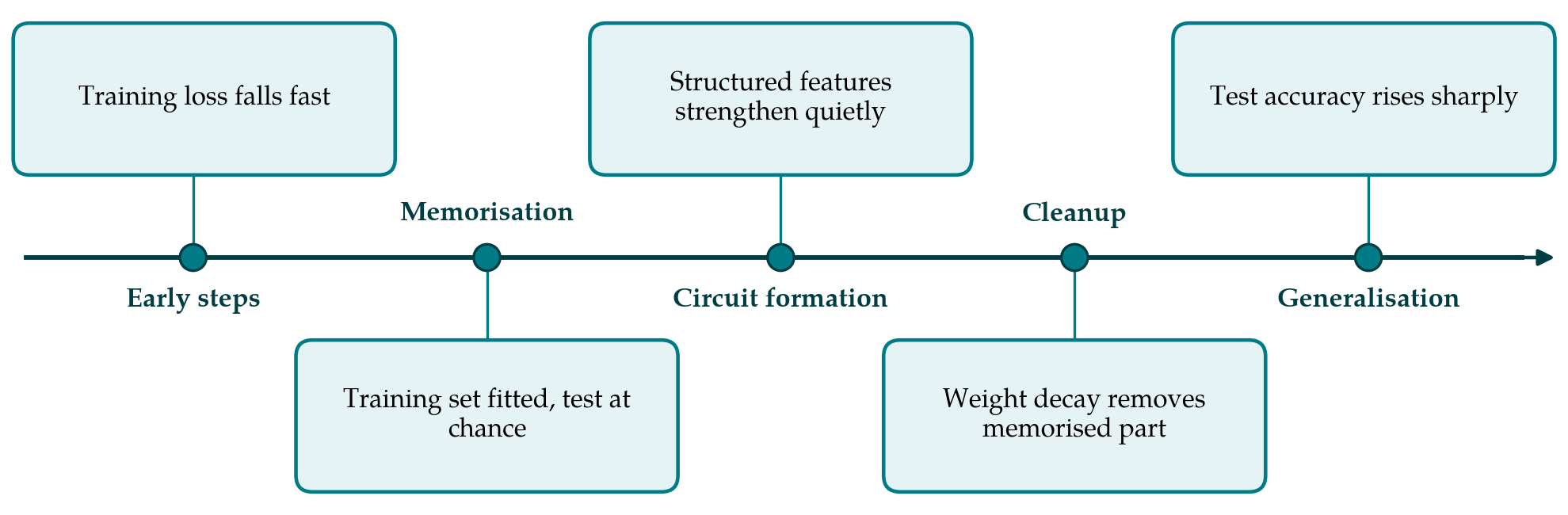
Figure 1: Sequence of training phases described in published accounts of grokking on modular arithmetic

3. Explanations on Offer

Several accounts of the delay have been published, and they are more complementary than they first appear. Table 1 lists them with the mechanism each emphasises and the prediction that distinguishes it.

Table 1: Published accounts of delayed generalisation and what each emphasises
Account	Mechanism emphasised	Distinctive prediction
Representation learning (Liu et al., 2022)	Generalisation waits for structured embeddings to form	Phase diagram with a narrow favourable region of hyperparameters
Weight norm (Liu et al., 2023)	Train and test losses favour different weight norms	Delay shrinks or grows with initialisation scale
Progress measures (Nanda et al., 2023)	Fourier circuit grows, then memorisation is cleaned up	Hidden measures move smoothly during the plateau
Circuit efficiency (Varma et al., 2023)	Generalising circuit gives larger logits per unit of norm	A critical dataset size; reversal if data are reduced
Slingshot (Thilak et al., 2022)	Cyclic instability of adaptive optimisers without weight decay	Generalisation coincides with spikes in last-layer norm

Liu et al. (2022) treat the problem as one of representation learning and map out regions of hyperparameter space in which a network generalises promptly, generalises late, only memorises, or fails to train. In a later paper the same group attribute the delay to a mismatch between the weight norms at which training loss and test loss are low, and show that the effect can be induced on tasks beyond arithmetic by starting from large weights (Liu et al., 2023). Varma et al. (2023) argue that the network holds two circuits, one that memorises and one that generalises, and that weight decay favours whichever produces the required outputs at lower parameter norm. Since memorising more examples costs more norm and generalising does not, there is a dataset size above which the generalising circuit wins.

Thilak et al. (2022) report the effect without explicit weight decay and connect it to a recurring instability of adaptive optimisers. A related line of theory shows that gradient descent on separable data keeps moving towards a large-margin solution long after training error is zero, and does so slowly (Soudry et al., 2018). What these accounts share is the view that a simpler solution is preferred, by explicit or implicit regularisation, and takes much longer to reach than the memorising one.

4. Observations for Reproducing the Effect

Four practical points follow from reading these papers together. The first is that the delay is a property of a configuration and not of the task alone. Training fraction, the strength of weight decay, the scale of initialisation and the choice of optimiser each move the onset of generalisation, and a small change can turn a long delay into none or into a run that never generalises. Weight decay should be specified exactly, including whether it is decoupled from the adaptive update as in AdamW (Loshchilov and Hutter, 2019), because the two forms regularise differently.

The second point is that loss and accuracy are the least informative quantities to record. Total weight norm, the norm of individual layers, and where a mechanism is known, measures tied to it, reveal movement during the plateau that the headline curves hide. The third is a matter of presentation: because the delay spans orders of magnitude, curves should be drawn on a logarithmic step axis, and a linear axis exaggerates the abruptness of the transition. The fourth is that several seeds are needed before any statement about timing is made, since the step at which generalisation appears varies between runs with identical settings.

5. What Small Models Can and Cannot Show

Modular arithmetic is attractive because the full input space is small, the correct algorithm is known, and a one-layer network can be understood completely. The same features limit what can be inferred. The task has an exact, compact solution, and natural data rarely do; the data are free of label noise; and the networks are far smaller than those in use. Barak et al. (2022) found a comparable pattern of hidden progress when networks learn sparse parities, which suggests the behaviour is not peculiar to one task, but that is still an algorithmic problem.

It would therefore be unsafe to conclude that large models trained on language or images will generalise if only they are trained long enough. The better-supported lesson is narrower. A flat validation curve does not prove that nothing is changing inside the network, and early stopping on such a curve can end training before a slower, more general solution has formed.

6. Conclusion

Grokking on modular arithmetic is now among the best-understood training phenomena in deep learning, largely because the task is small enough to be taken apart. The published explanations converge on a competition between a quick memorising solution and a slower, more economical generalising one, with regularisation deciding the outcome. For those who study it, the configuration matters as much as the task, internal measures matter more than accuracy, and caution is warranted in carrying conclusions to larger systems.

Conflict of interest

To be declared by the author(s) before publication.

Funding

To be declared by the author(s) before publication.

References

[1] Barak, B., Edelman, B.L., Goel, S., Kakade, S., Malach, E. and Zhang, C. Hidden progress in deep learning: SGD learns parities near the computational limit. Advances in Neural Information Processing Systems 35 (2022).
[2] Belkin, M., Hsu, D., Ma, S. and Mandal, S. Reconciling modern machine-learning practice and the classical bias-variance trade-off. Proceedings of the National Academy of Sciences https://doi.org/10.1073/pnas.1903070116 116(32), 15849-15854 (2019).
[3] Liu, Z., Kitouni, O., Nolte, N., Michaud, E.J., Tegmark, M. and Williams, M. Towards understanding grokking: An effective theory of representation learning. Advances in Neural Information Processing Systems 35 (2022).
[4] Liu, Z., Michaud, E.J. and Tegmark, M. Omnigrok: Grokking beyond algorithmic data. Proceedings of the International Conference on Learning Representations (2023).
[5] Loshchilov, I. and Hutter, F. Decoupled weight decay regularization. Proceedings of the International Conference on Learning Representations (2019).
[6] Nakkiran, P., Kaplun, G., Bansal, Y., Yang, T., Barak, B. and Sutskever, I. Deep double descent: Where bigger models and more data hurt. Proceedings of the International Conference on Learning Representations (2020).
[7] Nanda, N., Chan, L., Lieberum, T., Smith, J. and Steinhardt, J. Progress measures for grokking via mechanistic interpretability. Proceedings of the International Conference on Learning Representations (2023).
[8] Power, A., Burda, Y., Edwards, H., Babuschkin, I. and Misra, V. Grokking: Generalization beyond overfitting on small algorithmic datasets. arXiv preprint arXiv:2201.02177 (2022).
[9] Soudry, D., Hoffer, E., Nacson, M.S., Gunasekar, S. and Srebro, N. The implicit bias of gradient descent on separable data. Journal of Machine Learning Research 19(70), 1-57 (2018).
[10] Thilak, V., Littwin, E., Zhai, S., Saremi, O., Paiss, R. and Susskind, J. The slingshot mechanism: An empirical study of adaptive optimizers and the grokking phenomenon. arXiv preprint arXiv:2206.04817 (2022).
[11] Varma, V., Shah, R., Kenton, Z., Kramár, J. and Kumar, R. Explaining grokking through circuit efficiency. arXiv preprint arXiv:2309.02390 (2023).
[12] Zhang, C., Bengio, S., Hardt, M., Recht, B. and Vinyals, O. Understanding deep learning requires rethinking generalization. Proceedings of the International Conference on Learning Representations (2017).

Article metrics

0 total accesses since publication. 0 citing articles have been indexed to date.