1. Introduction
Almost every report on a nanomaterial states a particle size, and size is written into the common definitions of a nanomaterial as a length scale below about one hundred nanometres (ISO, 2015). Yet a size value on its own is nearly uninterpretable, because it depends on the quantity measured, the weighting applied and the method used. Two laboratories can characterise the same powder and publish sizes that differ by a factor of several without either being wrong, which undermines comparison across studies and the dose metrics used in nanotoxicology (Oberdörster et al., 2005).
The two most common methods illustrate the problem. Dynamic light scattering infers a hydrodynamic diameter from fluctuations in scattered light and is quick, inexpensive and applicable to a dispersion in situ (Berne and Pecora, 2000). Because the scattered intensity of a small particle rises steeply with its size, the method is strongly weighted towards the largest particles and towards any dust or aggregates, and the common cumulants analysis assumes a single population of spheres (ISO, 2017). Electron microscopy measures the geometric size of individual particles directly and reveals shape, but it samples a tiny fraction of the material, requires drying that can alter the state of the sample, and gives a number-weighted result that is sensitive to how particles are counted (ISO, 2019).
Because the weaknesses of the two methods are largely complementary, using them together is a natural response, and the idea is not new. What is often missing is a defined procedure that says how to combine them, how to convert between their different weightings so the numbers can be compared, and how to report the outcome so that another laboratory can reproduce it. This article sets out such a procedure. It is a proposal built from established techniques and international standards. It does not report measurements of its own, and it has not been validated here.
2. Background
A size distribution can be weighted by number, by surface area, by volume or by scattered intensity, and the mean of each weighting differs. For a distribution with any spread the intensity mean exceeds the volume mean, which exceeds the number mean, so that part of the apparent disagreement between methods is simply a difference of weighting and not of measurement (ISO, 2008). A further quantity, the polydispersity index returned by the cumulants fit in light scattering, summarises the width of the distribution but is frequently reported without stating that a value above about 0.7 means the cumulants model does not apply (ISO, 2017).
The guidance needed already exists in scattered form. The international standard on dynamic light scattering specifies how to run and fit the measurement; the standard on sizing by image analysis in electron microscopy specifies how many particles to count and how to measure them; and the standards on representing particle size distributions define the weightings and their conversion (ISO, 2019; ISO, 2008). Reviews of nanoparticle characterisation have repeatedly urged the use of more than one orthogonal method and the full reporting of conditions (Mourdikoudis et al., 2018). Other orthogonal methods exist, among them nanoparticle tracking analysis, whose strengths and limits for sizing were set out carefully by Filipe et al. (2010); the same reconciliation logic would extend to them. The contribution here is to assemble the two most common methods into one ordered procedure with the reconciliation step made explicit.
3. The Proposed Procedure
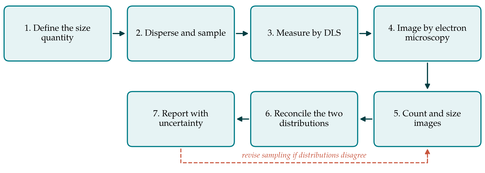
The procedure has seven steps, listed in Table 1 and shown as a flow in Figure 1. Each is described below with the standard it draws on and the record it should produce. The procedure is proposed and has not been validated on real specimens in this article.
| Step | Technique or basis | Output recorded |
|---|---|---|
| 1. Define the size quantity | Choose number or volume weighting ISO, 2008 | Quantity and weighting stated in advance |
| 2. Disperse and sample | Stated medium, sonication, concentration | Preparation protocol |
| 3. Measure by DLS | Cumulants and distribution fit ISO, 2017 | Z-average, PDI, fit residuals |
| 4. Image by electron microscopy | Counted particles ISO, 2019 | Micrographs and magnification calibration |
| 5. Count and size images | Measure a defined particle dimension | Number-weighted distribution |
| 6. Reconcile distributions | Convert weightings and compare ISO, 2008 | Agreement or documented discrepancy |
| 7. Report with uncertainty | State distribution and spread | Result with uncertainty budget |
3.1. Step 1: Define the size quantity before measuring
The first decision is what is to be reported, because it determines what counts as agreement later. A number-weighted median geometric diameter and an intensity-weighted hydrodynamic diameter are different physical quantities, and a procedure that does not fix the target quantity in advance invites the familiar practice of quoting whichever method gives the preferred number. The choice should follow the use: a number distribution suits counting and definitions of a nanomaterial, a volume or surface distribution suits dose and reactivity.
3.2. Step 2: Disperse and sample in a stated way
Measured size depends on the state of dispersion as much as on the particles. The medium, its ionic strength and pH, the concentration, and any sonication must be fixed and recorded, because aggregation changes with all of them. The same stock dispersion should feed both measurements, prepared at the same time, so that the two methods see the same material rather than two differently aged suspensions. Sampling from a settling or aggregating suspension is a known source of bias and should be controlled by mixing immediately before each aliquot is taken.
3.3. Step 3: Measure by dynamic light scattering
The scattering measurement follows the international standard: a transparent, dust-free dilution, a controlled temperature, and replicate runs (ISO, 2017). Both the cumulants result, giving the z-average diameter and polydispersity index by the method of cumulants (Koppel, 1972), and a regularised distribution fit such as the constrained inversion of Provencher (1982) should be recorded, together with the correlation function and its residuals so that fit quality can be judged. A high polydispersity index is reported as a warning that the sample is not suited to the assumptions of the method rather than concealed in a single mean.
3.4. Step 4: Image by electron microscopy
Transmission or scanning electron microscopy provides the geometric sizes. The magnification is calibrated against a certified reference, and fields are selected without reference to particle size to avoid the temptation to image attractive regions. Because drying can cause aggregation and flattening, the preparation method is recorded, and where the dried state is in doubt a cryogenic method is preferable (ISO, 2019).
3.5. Step 5: Count and size the images
A defined dimension, such as the area-equivalent circular diameter, is measured for a counted number of particles large enough that the distribution is stable, with the counting rules for touching and partly visible particles stated. Image analysis should be checked against manual measurement on a subset, because automatic segmentation can merge or split particles. The output is a number-weighted size distribution with its count.
3.6. Step 6: Reconcile the two distributions
This is the step that distinguishes the procedure from running two methods side by side. The number-weighted microscopy distribution is converted to an intensity or volume weighting, using the defined relationships between weightings and, for the scattering comparison, a scattering model appropriate to the particle size and refractive index (ISO, 2008). If the converted microscopy result and the scattering result then agree within their uncertainties, the sample is well described by a single population and the result is secure. If they disagree, the discrepancy is itself informative: a scattering size much larger than the converted microscopy size usually indicates aggregates or a small number of large particles that dominate the scattered intensity, and the procedure returns to sampling and dispersion rather than to averaging the two numbers. The sensitivity of the measured size to the state of dispersion is well documented for toxicology specimens by Jiang et al. (2009), whose work underlines why the same stock and a recorded preparation matter.
3.7. Step 7: Report with an uncertainty budget
The result is reported as a distribution, not a single diameter, with the chosen weighting, the median and a measure of spread, the number of particles counted and the scattering conditions. An uncertainty budget is assembled following the general guidance on measurement uncertainty, including contributions from calibration, sampling, counting statistics and the weighting conversion (JCGM, 2008). The report should allow another laboratory to repeat the measurement and obtain a value within the stated uncertainty.
4. Fitting the Procedure to Practice
The procedure uses only instruments that a materials laboratory with access to electron microscopy already has, and it adds method time rather than equipment. The main cost is the microscopy counting and the reconciliation, which can be supported by freely available image analysis software. For routine quality control of a well-behaved product the full reconciliation need be done only during method validation, after which a faster single-method check may suffice, provided the validation established that the two methods agree for that material. The procedure is most valuable for new, polydisperse or non-spherical materials, which are exactly the cases where single-method sizing misleads.
Two practical safeguards keep the method honest. Fields for microscopy are chosen before the particles in them are sized, by moving to predefined stage positions rather than by searching for a pleasing image, so that the count is not biased towards the size the operator expects. And the scattering dilution is prepared and filtered so that a single stray aggregate does not dominate the intensity signal; a run whose correlation function shows a slow second decay is repeated rather than reported. Neither safeguard needs new equipment, and both address the commonest ways in which a sizing result is quietly skewed before any analysis begins.
5. Limitations and What Remains to Be Shown
Several limitations are intrinsic. The weighting conversion from a number distribution to an intensity distribution amplifies the tail of large particles, so a microscopy count that misses rare large particles will convert to a scattering size that is too small, and no amount of reconciliation recovers particles that were never imaged. The scattering model used in the conversion assumes a shape and a refractive index that may be uncertain. For strongly non-spherical or core-shell particles neither a hydrodynamic diameter nor a single geometric dimension fully describes the object.
Because this is a proposal, its properties have not been demonstrated. Before adoption it would need to be applied to reference materials of known size distribution, including a certified monodisperse latex and a deliberately polydisperse or bimodal mixture, to show that the reconciliation detects known discrepancies and that different operators obtain consistent results. An interlaboratory comparison would be the proper test of reproducibility. Until such studies are done the procedure is a structured way to use two methods well, not a validated measurement standard.
6. Conclusion
Reproducible nanoparticle sizing requires more than a good instrument; it requires agreement in advance on what is being measured and an explicit way to reconcile methods that weight the distribution differently. The seven-step procedure proposed here combines dynamic light scattering and electron microscopy by converting their results to a common weighting and treating a disagreement as a signal to investigate sampling rather than a number to average. It draws throughout on existing international standards. Its value in practice is an empirical matter that the validation studies described above would settle, and that practitioners are well placed to carry out. Adopting even the reporting discipline it describes, namely stating the quantity, the weighting, the number of particles counted and the scattering conditions, would make published sizes more comparable than they are now, which is a benefit available before any formal validation is complete.
Conflict of interest
To be declared by the author(s) before publication.
Funding
To be declared by the author(s) before publication.