1. Introduction
The dose-response curve is the basic quantitative object of pharmacology and toxicology. From it come the potency of a compound, its maximal effect, the steepness of the transition between them, and the doses taken forward into later studies. In early research the curve is nearly always estimated from little data. The principle of reduction, one of the three Rs set out by Russell and Burch (1959), obliges investigators to use no more animals than the question requires, and practical constraints on compound supply and time push in the same direction. A typical in vivo experiment has a vehicle group and a few dose groups with a small number of animals in each, and the in vitro equivalents are often not much larger once the true unit of replication is counted.
Small experiments are not in themselves a fault, but they strain the statistical methods routinely applied to them. Low power and inflated effect estimates have been documented across the preclinical sciences (Button et al., 2013), and nonlinear curve fitting adds difficulties of its own. Bayesian hierarchical modelling has become the main proposal for analysing such data more stably, because it lets related curves inform one another and admits external information in a controlled way. This article reviews that proposal: what the models are, what they require of the analyst, and where their limits lie.
2. Approach of This Review
The article is a narrative review. It draws on standard texts in Bayesian and multilevel modelling (Gelman and Hill, 2007; Gelman et al., 2013), on methodological papers concerning priors, historical data and computation, and on guidance from the toxicological risk assessment community. The literature was not searched systematically, and the selection favours sources that a practising analyst can act on. Clinical dose-finding designs are outside the scope except where their methods have been carried over to laboratory work.
3. Why Small Dose-Response Studies Are Hard to Analyse
Two separate problems arise when a curve is fitted to a small experiment. One concerns the curve, the other the structure of the data.
3.1. Curve fitting with few dose groups
The usual model is the four-parameter log-logistic or Hill function, with a lower asymptote, an upper asymptote, a midpoint (the ED50 or EC50) and a slope (Ritz et al., 2015). Estimating four parameters well requires doses that define both plateaus as well as the rising part of the curve, a condition spelled out in the practical guidelines of Sebaugh (2011). When the top doses do not reach the plateau, or only one dose falls on the slope, the likelihood is nearly flat in some directions. Optimisers then fail to converge or return estimates at the edge of the allowed range, the midpoint and slope become strongly correlated, and confidence intervals based on large-sample theory cannot be trusted. Analysts often respond by fixing an asymptote or the slope at a convenient value, which is an informal prior applied without acknowledgement and without any allowance for uncertainty.
3.2. Nested data and the experimental unit
Preclinical data are rarely a simple random sample. Several measurements come from one animal, several animals from one litter or cage, several wells from one plate, and several plates from one day's work. Treating every measurement as independent overstates the amount of information and is the error known as pseudoreplication (Lazic, 2010). The remedy is to identify the experimental unit, the entity that was independently assigned to a dose, and to model variation above and below it explicitly (Lazic et al., 2018). A model with terms for animal, plate or batch is already a hierarchical model, whatever name is given to it, and the ARRIVE 2.0 reporting guidelines now ask authors to state the experimental unit for exactly this reason (Percie du Sert et al., 2020).
4. The Hierarchical Formulation
The central idea is older than its current popularity. Lindley and Smith (1972) showed that when the parameters of several similar regressions are regarded as exchangeable draws from a common distribution, the estimate for each one is pulled towards the common mean by an amount that depends on how precisely it is determined by its own data. Units with little data are pulled strongly and units with plentiful data hardly at all. This behaviour is called partial pooling or shrinkage. It sits between two extremes that are both unsatisfactory in small studies: fitting every curve separately, which is unstable, and fitting one curve to everything, which ignores real differences.
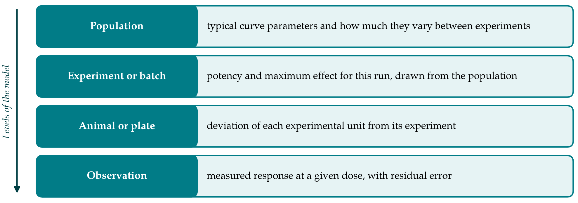
In a dose-response setting the model is built in levels, as Figure 1 shows. At the bottom, each observation is the value of the Hill function at the given dose plus residual error. The parameters of that function belong to an experimental unit, and unit-level parameters vary around the values for their experiment or batch. Those in turn vary around population values. Not every parameter needs to vary at every level. A common and defensible choice lets the midpoint, on the logarithmic scale, and the maximal effect differ between experiments while the slope is shared or allowed only modest variation, since the slope is the parameter least well determined by sparse data. The textbook bioassay example in Gelman et al. (2013), in which a few animals are tested at each of four dose levels, shows in miniature how much a single small experiment can and cannot say.
The gain is practical. A plate in which the top concentration failed, or an animal cohort that did not reach the plateau, still yields a usable curve, because the missing information about the asymptote is borrowed from sister experiments. Uncertainty about the population parameters is carried through to every derived quantity, so the interval for a potency ratio or a predicted response at an untested dose reflects all sources of variation in the model. The same structure extends naturally to several compounds tested in a common assay, where compound-level potencies are themselves given a distribution.
5. Priors When Groups Are Few
A hierarchical model needs prior distributions at the top level, and in small studies these matter. The main components of a model and the concern each raises are summarised in Table 1.
| Component | Common choice | Concern in small studies | Sources |
|---|---|---|---|
| Mean function | Four-parameter log-logistic (Hill) curve | Plateaus poorly defined by the doses tested | Ritz et al., 2015; Sebaugh, 2011 |
| Group-level structure | Varying midpoint and maximum; shared slope | Too many varying terms for the number of groups | Gelman and Hill, 2007 |
| Prior on between-group scale | Half-normal, half-t or half-Cauchy | Posterior sensitive to the prior when groups are few | Gelman, 2006; Polson and Scott, 2012 |
| Historical controls | Meta-analytic-predictive or power prior | Conflict between past and current data | Neuenschwander et al., 2010; Schmidli et al., 2014 |
| Model uncertainty | Averaging over candidate curve shapes | Data cannot discriminate between shapes | Hoeting et al., 1999; Wheeler and Bailer, 2007 |
| Model checking | Prior and posterior predictive checks; cross-validation | Few observations against which to check | Gabry et al., 2019; Vehtari et al., 2017 |
5.1. Between-group variation
The parameter that governs how much pooling occurs is the standard deviation of the group-level distribution. With many groups the data determine it and the prior is of little consequence. With three or four experiments they do not, and the prior can dominate. Gelman (2006) examined this case and showed that the inverse-gamma priors once used by default as supposedly non-informative choices behave badly, because the posterior remains sensitive to the arbitrary constant in the prior when the true variance may be near zero. He recommended priors placed directly on the standard deviation, such as a uniform or a half-t distribution, with a weakly informative scale when groups are few. Polson and Scott (2012) gave further theoretical support for the half-Cauchy. In laboratory work the scale can usually be set from knowledge of the assay: how much the midpoint is known to move from run to run is something experienced laboratories can state, at least roughly.
Priors on the curve parameters themselves are less contentious. The midpoint can reasonably be expected to lie within or near the range of doses tested, the asymptotes are bounded by the measurement scale and by control wells or vehicle animals, and the slope is positive and seldom extreme. Weakly informative priors that encode these facts exclude absurd curves without constraining plausible ones, and they are what makes the sampler stable when individual curves are incomplete.
5.2. Historical information
Laboratories that run an assay repeatedly accumulate data on control groups and reference compounds, and using those data can reduce the number of animals needed in a new study. Two formal devices are in common use. The power prior raises the likelihood of the historical data to a power between zero and one, which discounts it relative to current data (Ibrahim and Chen, 2000). The meta-analytic-predictive approach fits a hierarchical model to the historical studies and takes the predictive distribution for a new study as the prior (Neuenschwander et al., 2010). Because past and present may differ, Schmidli et al. (2014) proposed mixing that prior with a vague component so that it gives way when the new data disagree. Both methods were developed for clinical trials, and both transfer directly to preclinical controls provided the historical experiments are comparable in strain, protocol and measurement.
6. Computation and Model Checking
Fitting these models once required custom code. General-purpose software now does the work. Stan implements Hamiltonian Monte Carlo with adaptive tuning and has become a standard engine for hierarchical models (Carpenter et al., 2017), and the brms package allows nonlinear multilevel models, Hill curves included, to be specified in R formula syntax and passed to Stan (Bürkner, 2017). Small hierarchical data sets are, perhaps unexpectedly, among the harder cases computationally. When the between-group standard deviation is poorly determined, the posterior has a funnel shape that samplers explore badly, and the software reports divergent transitions. The standard remedy is the non-centred parameterisation, in which group effects are expressed as scaled standard deviates (Papaspiliopoulos et al., 2007). Sampler warnings should be resolved and not ignored, since they indicate that the reported intervals may be wrong.
A fitted model then has to be checked. Simulating data from the prior alone shows whether the priors imply sensible curves before any data are seen, and simulating from the posterior shows whether the model can reproduce the observed pattern of responses across doses; both are part of the graphical workflow described by Gabry et al. (2019). Competing structures, for example shared versus varying slopes, can be compared by approximate leave-one-out cross-validation (Vehtari et al., 2017), though with few experimental units such comparisons are themselves uncertain and should not be over-read. A sensitivity analysis that refits the model under a wider and a narrower prior for the between-group scale is the single most informative check in a small study.
7. Benchmark Dose Estimation
Toxicological risk assessment offers the most developed regulatory use of these ideas. Crump (1984) proposed replacing the no-observed-adverse-effect level, which depends heavily on the doses chosen and the group size, with a benchmark dose defined as the dose producing a specified change in response, reported with a lower confidence bound. Because several curve shapes usually fit toxicity data about equally well and give different benchmark doses, averaging across models was introduced to carry that uncertainty into the result (Wheeler and Bailer, 2007), following the general framework of Bayesian model averaging (Hoeting et al., 1999). The current guidance of the European Food Safety Authority recommends a Bayesian approach with model averaging as the preferred method for deriving a reference point (EFSA Scientific Committee, 2022). Hierarchical structure enters when data from several studies, sexes or related endpoints are analysed together, so that each sparse data set is supported by the others.
8. Limits and Open Questions
The method has costs and conditions. Partial pooling assumes that the units being pooled are exchangeable, meaning that nothing known beforehand distinguishes one from another. If one experiment used a different strain or one compound belongs to a different chemical class, that assumption fails unless the difference is put into the model as a covariate. Shrinkage also pulls unusual units towards the centre, and an unusual unit is sometimes the discovery. A compound that is truly far more potent than its relatives will be estimated as somewhat less so, and the analyst should look at unpooled estimates alongside pooled ones before concluding that nothing stands out.
Dependence on the prior cannot be removed when groups are few, only made visible. Reports should state every prior, give the reasoning for the between-group scale, show the sensitivity analysis and identify the experimental unit, in the spirit of the reporting recommendations long made for Bayesian analyses in health research (Spiegelhalter et al., 2004). Where a decision rule will be applied repeatedly, for instance a criterion for advancing compounds, its long-run error rates under plausible scenarios can be examined by simulation before the method is adopted. Published evaluations of that kind for preclinical dose-response settings are still uncommon, and guidance on default priors for particular assay types is thinner than for clinical trials. These are the areas in which further methodological work would be most useful to laboratories.
9. Conclusion
Hierarchical Bayesian models suit the conditions under which preclinical dose-response data are produced: few units, incomplete curves, nested measurements and a body of related experiments. They stabilise estimation by sharing information, represent the experimental design honestly and express uncertainty in the quantities that matter for decisions. Their results in small studies depend on assumptions about between-group variation and exchangeability that the data cannot fully test. Used with stated priors, sensitivity analysis and proper checks, they are a sound replacement for curve-by-curve fitting. Used as a black box, they move the fragility of small studies from the optimiser to the prior.
Conflict of interest
To be declared by the author(s) before publication.
Funding
To be declared by the author(s) before publication.