1. Introduction
A wearable biosensor that harvests its own energy lives on a strict allowance. A thermoelectric generator on the skin, a small photovoltaic cell under indoor light or a coil in the field of a nearby reader delivers power that is small, intermittent and available at a low voltage (Paradiso and Starner, 2005). Interface circuits can now start from thermoelectric outputs of a few tens of millivolts (Ramadass and Chandrakasan, 2011), yet whatever they deliver must be shared between sensing, conversion and a radio link.
The first amplifier of the front end carries most of that burden. It faces a skin electrode or an electrochemical cell, sources that combine small signals with large and slowly drifting offsets, and it determines the noise of the whole chain. Operating its transistors below threshold, in weak inversion, is the accepted route to low power: the region offers the largest transconductance for a given bias current and tolerates supply voltages well under one volt (Vittoz and Fellrath, 1977). The price is paid in speed, matching and sensitivity to temperature, and a designer who treats weak inversion as strong inversion with smaller numbers will be surprised on all three counts.
This article proposes a six-step procedure for designing a sub-threshold operational amplifier, in practice usually an operational transconductance amplifier (OTA), for the front end of a battery-free wearable biosensor. It draws on the published work on micropower biopotential and neural amplifiers, on the gm/ID sizing method and on the device physics of weak inversion. No amplifier has been fabricated or measured for this article. What is offered is the ordering of the decisions, the reasoning behind each and a statement of what remains to be demonstrated.
2. Background
Three bodies of knowledge feed the procedure: how a MOS transistor behaves below threshold, what a wearable sensor asks of its amplifier, and what a harvested supply imposes.
2.1. Weak inversion in brief
In weak inversion the channel current flows by diffusion and depends exponentially on the gate voltage, much as collector current depends on base-emitter voltage in a bipolar transistor. The transconductance is then proportional to the drain current and equals ID/(nUT), where UT = kT/q is the thermal voltage, about 26 mV at room temperature, and n is the slope factor, somewhat greater than one in bulk CMOS. The ratio gm/ID therefore reaches its ceiling of 1/(nUT) in this region and falls steadily as the device is pushed towards strong inversion. The EKV model describes the transition between the regions with a single continuous expression and introduced the inversion coefficient as a measure of where a device sits (Enz et al., 1995).
Two consequences matter for amplifier design. A device saturates once its drain-source voltage exceeds a few thermal voltages, roughly 100 mV, so several transistors can be stacked under a supply of half a volt. Against that, the high gm/ID that makes the input pair efficient also makes current mirrors poor: a given threshold mismatch produces a current error proportional to gm/ID, and threshold mismatch itself shrinks only with the square root of gate area (Pelgrom et al., 1989). Weak inversion devices are also wide, slow and exponentially sensitive to temperature, which is why the choice of inversion level is made device by device and not once for the whole circuit (Binkley, 2008).
2.2. What the sensor asks of the amplifier
Wearable sensors fall into two electrical families. Biopotential electrodes for the electrocardiogram, electromyogram or electroencephalogram present signals from microvolts to a few millivolts at frequencies from a fraction of a hertz to a few kilohertz, superimposed on electrode offsets that can be hundreds of times larger than the signal (Webster, 2010). Electrochemical sensors for sweat or interstitial fluid are either potentiometric, where an ion-selective electrode produces a slowly varying voltage behind a very high source impedance, or amperometric, where an enzyme electrode held at a fixed potential produces a small current (Bandodkar and Wang, 2014; Gao et al., 2016). The first family needs a low-noise voltage amplifier that rejects offset. The second needs a buffer with negligible input current or a transimpedance stage within a potentiostat loop.
The circuit literature offers a well-tried pattern for the first family. Harrison and Charles (2003) placed an OTA inside a capacitive feedback network, so that the electrode offset is blocked by the input capacitors and the gain is fixed by a capacitor ratio, and used MOS-bipolar pseudo-resistors to set a very low high-pass corner without large passive components. Their amplifier became the reference point for later work, including the folded-cascode variant of Wattanapanitch et al. (2007), which restricted the current in the folding branches to bring the noise closer to the limit set by the input pair.
2.3. What the supply imposes
A harvested supply is low, noisy and finite. Rectifiers and boost converters leave ripple on it, and the storage capacitor droops between harvesting bursts. The amplifier therefore needs good supply rejection in the signal band, or a quiet local regulator whose own current is counted in the budget. Reference voltages and bias currents must come from circuits that work at the same low supply; references built entirely from sub-threshold MOSFETs, consuming a fraction of a microwatt, were demonstrated by Ueno et al. (2009). Analogue design at half a volt is feasible but changes the topology, as the body-input and gate-input OTAs of Chatterjee et al. (2005) showed.
3. The Proposed Procedure
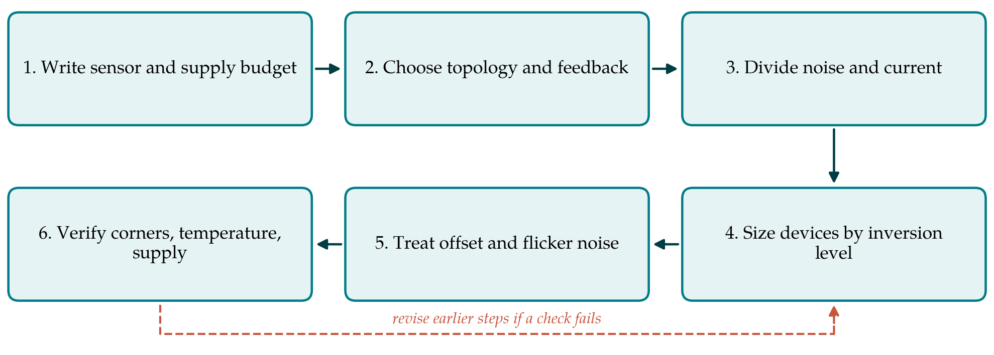
The procedure orders the design into six decisions, each of which constrains the next. Table 1 lists the steps with the main choice made and the record that should come out of each. Figure 1 shows the sequence and the return path taken when a late check fails. The method is proposed here as a way of organising published practice. It has not been validated by carrying a design through to silicon.
| Step | Main decision | Record produced |
|---|---|---|
| 1. Sensor and supply budget | Signal band, noise target, offset range, minimum supply, available current | One-page specification with duty cycle |
| 2. Topology and feedback | Feedback network for the sensor type; OTA stage count by headroom | Schematic outline with headroom count |
| 3. Noise and current split | Total current from the noise target; share given to the input pair | Branch currents and noise shares |
| 4. Sizing by inversion level | g /I and length for every device m D | Sizing table with inversion coefficients |
| 5. Low-frequency errors | Input device area; whether to chop or auto-zero | Offset and flicker noise estimate |
| 6. Verification | Corners, temperature, mismatch, supply ripple, start-up | Simulation report with the real bias circuit |
3.1. Step 1: Write the sensor and supply budget
The first output is a single page of numbers agreed before any transistor is drawn: signal band, smallest signal to be resolved, largest signal and offset to be tolerated, source impedance, minimum supply voltage at the end of a droop, and the average and peak current the harvester can sustain. For a biopotential channel the noise target should be set from the application and not from what the best published amplifier achieved, since each halving of input-referred noise costs roughly four times the current in a stage limited by thermal noise. The budget should also state the duty cycle, because an amplifier that must settle quickly after power-up is a different design from one that runs continuously.
3.2. Step 2: Choose the topology and the feedback network
The sensor family largely decides the feedback network: capacitive feedback for biopotentials, a unity-gain buffer for potentiometric electrodes, resistive or switched-capacitor transimpedance for amperometric cells. The OTA inside it is then chosen by counting headroom. A single-stage telescopic or folded-cascode OTA has one dominant pole at its output and is easy to stabilise with the load capacitance, but each cascode consumes a saturation voltage. A two-stage amplifier gives more swing and gain at low supply at the cost of a compensation network and a second branch of current. Below about half a volt neither cascodes nor a conventional tail source may fit, and the designer is led towards pseudo-differential, inverter-based or bulk-driven input stages with separate common-mode control (Chatterjee et al., 2005).
3.3. Step 3: Divide the noise and current budget
The noise efficiency factor introduced by Steyaert and Sansen (1987) compares the input-referred noise of an amplifier with that of a single bipolar transistor drawing the same total current over the same bandwidth. An ideal single device scores one, and practical differential CMOS amplifiers score above that. The factor is a convenient way to turn the noise target of step 1 into a total current and then to check how much of that current may be spent outside the input pair. A reasonable starting split gives the input devices the large majority of the supply current and requires that all other devices together add only a modest fraction to the input-referred thermal noise.
3.4. Step 4: Size each device by its inversion level
Sizing follows the gm/ID method of Silveira et al. (1996), in the lookup-table form developed by Jespers and Murmann (2017). For each transistor the designer picks a gm/ID value and a channel length, reads the corresponding current density from curves generated by simulating the foundry model, and obtains the width from the branch current. The input pair is placed deep in weak inversion, close to the maximum gm/ID, which makes it wide. Current-source loads and mirrors are deliberately placed in moderate or strong inversion with long channels, so that their transconductance, and hence their noise and mismatch contribution referred to the input, is several times smaller than that of the input pair.
Two checks close this step. The first is bandwidth: weak inversion gives a low transit frequency, and the large input devices add gate capacitance that attenuates the signal in a capacitive-feedback stage and raises the input-referred noise. The second is intrinsic gain at the chosen lengths, which short devices in a modern process may not supply. If the headroom of step 2 does not permit strong-inversion loads, source degeneration with resistors or with long-channel devices achieves a similar reduction of their noise contribution (Wattanapanitch et al., 2007).
3.5. Step 5: Deal with offset, flicker noise and mismatch
Biosignals sit in the band where flicker noise dominates. Because flicker noise falls with gate area, the wide input devices of step 4 help, and p-channel inputs are preferred in many processes for their lower flicker noise. When area alone is not enough, the established remedies are chopper stabilisation and auto-zeroing, whose principles and residual errors are set out by Enz and Temes (1996) and which have been applied to micropower biopotential amplifiers (Denison et al., 2007). Chopping moves offset and flicker noise out of the band but lowers the input impedance and creates ripple that must be filtered, so it should be adopted only when the budget shows a need. Offset is estimated from the area law for threshold mismatch and compared with the output swing available after gain.
3.6. Step 6: Verify against corners, temperature and supply
Weak inversion currents change by large factors between process corners and across the temperature range of skin-worn equipment, so the bias generator, not the amplifier, decides whether the design survives. Simulation should cover corners and temperature with the real bias circuit in place, Monte Carlo analysis of offset and of the pseudo-resistor corner frequency, supply rejection with the expected ripple spectrum, and the start-up transient from a discharged storage capacitor. A check that fails sends the designer back to an earlier step, most often the sizing of step 4 and sometimes the budget of step 1. Figure 1 shows this return path.
4. Fitting the Procedure to a Process and a Sensor
The procedure is independent of the technology node, but two choices depend on it. Older nodes with thicker gate oxide have negligible gate leakage and well-behaved long-channel devices, which suits amplifiers whose bandwidth is a few kilohertz at most. Finer nodes bring gate leakage that appears as input current, a serious matter for a potentiometric electrode. Where the process offers a deep n-well, body terminals can be used as second inputs or for threshold adjustment at low supply. For amperometric sensors the same OTA is reused as the control amplifier of the potentiostat, and step 1 must then include the cell capacitance, which loads the amplifier and governs stability.
5. Limitations and What Remains to Be Shown
The procedure has been assembled from published circuits and textbooks and has not been tested by applying it to a new amplifier, so its claims are of coherence and not of performance. Several things would need to be shown. One is that a designer following the six steps arrives at a noise efficiency comparable with the published state of the art without many iterations. Another is that the supply-rejection and start-up checks of step 6 predict behaviour under a real harvester, whose ripple and impedance are harder to model than a bench supply. A third concerns the electrode: skin contact impedance and motion artefact vary between wearers and over time, and no amplifier specification removes them.
The method is also silent on what follows the amplifier. An analogue-to-digital converter, a reference and a radio share the same harvested energy, and optimising the first stage in isolation can move the problem downstream. System-level allocation of the energy budget lies outside the scope of this article.
6. Conclusion
Sub-threshold operation gives the wearable front end its efficiency, and it rewards a designer who decides, transistor by transistor, where on the inversion scale each device should sit. The procedure proposed here starts from a written sensor and supply budget, selects topology by headroom, apportions noise with the noise efficiency factor, sizes by gm/ID, treats low-frequency errors explicitly and ends with verification that includes the bias circuit and the supply. Whether it shortens design time or improves results is a question for those who apply it to silicon.
Conflict of interest
To be declared by the author(s) before publication.
Funding
To be declared by the author(s) before publication.