1. Introduction
Thermal conductivity is among the harder material properties to measure well. Steady-state methods such as the guarded hot plate are capable of low uncertainty but need large, flat specimens and long settling times (Salmon, 2001). Transient methods trade some of that rigour for speed and convenience. The transient plane source technique introduced by Gustafsson (1991) uses a thin metal spiral as both heater and thermometer, clamped between two pieces of the specimen, and returns thermal conductivity and thermal diffusivity from a recording that lasts seconds to minutes. It is now the subject of an international standard (ISO, 2015) and is used across polymers, building materials, ceramics, battery components and insulation.
Ease of use has a cost. Papers that rely on the technique frequently report a conductivity with an uncertainty copied from the manufacturer's general specification, or with the standard deviation of a few repeat shots. Neither is an uncertainty in the sense of the Guide to the Expression of Uncertainty in Measurement, the GUM (JCGM, 2008a). Repeatability captures only random scatter under unchanged conditions. A general specification cannot know whether the probing depth stayed inside the specimen, whether contact was good, or how well the specific heat was known.
This article sets out a procedure by which a laboratory can build an uncertainty statement for an individual transient plane source result. It is written for users of commercial instruments who have access to the recorded transient and to ordinary scripting tools. The procedure is proposed on the basis of the published theory of the method and of the metrological guidance documents; it has not been applied to experimental data here, and what would be needed to validate it is stated near the end.
2. Background
Two bodies of material underlie the procedure: the conduction model on which the technique rests, and the framework within which measurement uncertainty is evaluated.
2.1. The measurement model
The sensor is a double spiral etched from nickel foil and sandwiched between thin insulating films, usually polyimide. A constant current heats it, and its resistance, which rises with temperature, is recorded through a bridge. The technique grew out of the transient hot-strip method (Gustafsson et al., 1979). In the ideal model the spiral is replaced by a set of concentric ring sources in an infinite homogeneous medium, and the solution of the conduction equation (Carslaw and Jaeger, 1959) gives the mean temperature rise of the sensor as ΔT(τ) = P0 D(τ) / (π3/2 r k). Here P0 is the heating power, r the sensor radius, k the thermal conductivity, D(τ) a tabulated dimensionless function and τ = (αt)1/2/r the dimensionless time formed with the thermal diffusivity α (He, 2005).
Because τ contains the unknown diffusivity, the evaluation is iterative. The software searches for the diffusivity, and for a small time correction, that make the recorded temperature rise a straight line against D(τ); the conductivity then follows from the slope. The earliest points are discarded, because they are dominated by the insulating film and the contact between sensor and specimen, and the recording must end before the heat reaches any outer boundary. Bohac et al. (2000) examined how the choice of time window affects the sensitivity of the fit to each parameter and showed that both properties are well determined only when the window spans a suitable range of dimensionless time.
Variants of the basic experiment exist for slabs, thin films and anisotropic materials (Gustavsson et al., 1994; Log and Gustafsson, 1995). Several of them require the volumetric heat capacity as an input, which adds a further measured quantity to the model.
2.2. The uncertainty framework
The GUM expresses a result as a function of input quantities, assigns each input a standard uncertainty from statistical analysis of repeated observations (Type A) or from other knowledge (Type B), and combines them through first-order sensitivity coefficients (JCGM, 2008a; Taylor and Kuyatt, 1994). The approach assumes that the model is nearly linear over the range of the uncertainties. Supplement 1 replaces the linear combination with numerical propagation of full probability distributions by Monte Carlo sampling and is recommended when linearity or normality is doubtful (JCGM, 2008b). A fitted, iterative model such as that of the transient plane source is a natural candidate for the second route. The engineering literature on experimental uncertainty offers the same ideas in different vocabulary (Moffat, 1988).
3. The Proposed Procedure
The procedure has seven steps, shown in sequence in Figure 1. Table 1 lists the input quantities that the second and third steps are concerned with, since identifying them is where most of the judgement lies. The steps are then described in turn.
| Input quantity | How it enters the result | Basis for its uncertainty |
|---|---|---|
| Heating power | Scales conductivity directly through the slope | Calibration of current and sensor resistance; lead losses |
| Temperature coefficient of resistance | Converts resistance change to temperature rise | Sensor calibration certificate; dependence on temperature |
| Sensor radius | Enters the slope and the dimensionless time | Manufacturing tolerance; effective versus nominal radius |
| Time window and time correction | Fixes which points are fitted and the fitted diffusivity | Repeat evaluation over alternative windows |
| Sensor heat capacity and insulation | Delays the early response; biases low-conductivity results | Model with and without correction; reference material |
| Contact between sensor and specimen | Adds an initial offset that the fit must absorb | Remounting the specimen between repeats |
| Volumetric heat capacity | Required input in slab and anisotropic modes | Uncertainty of the separate calorimetric measurement |
| Specimen temperature drift | Superimposes a baseline on the transient | Recorded drift before the heating pulse |
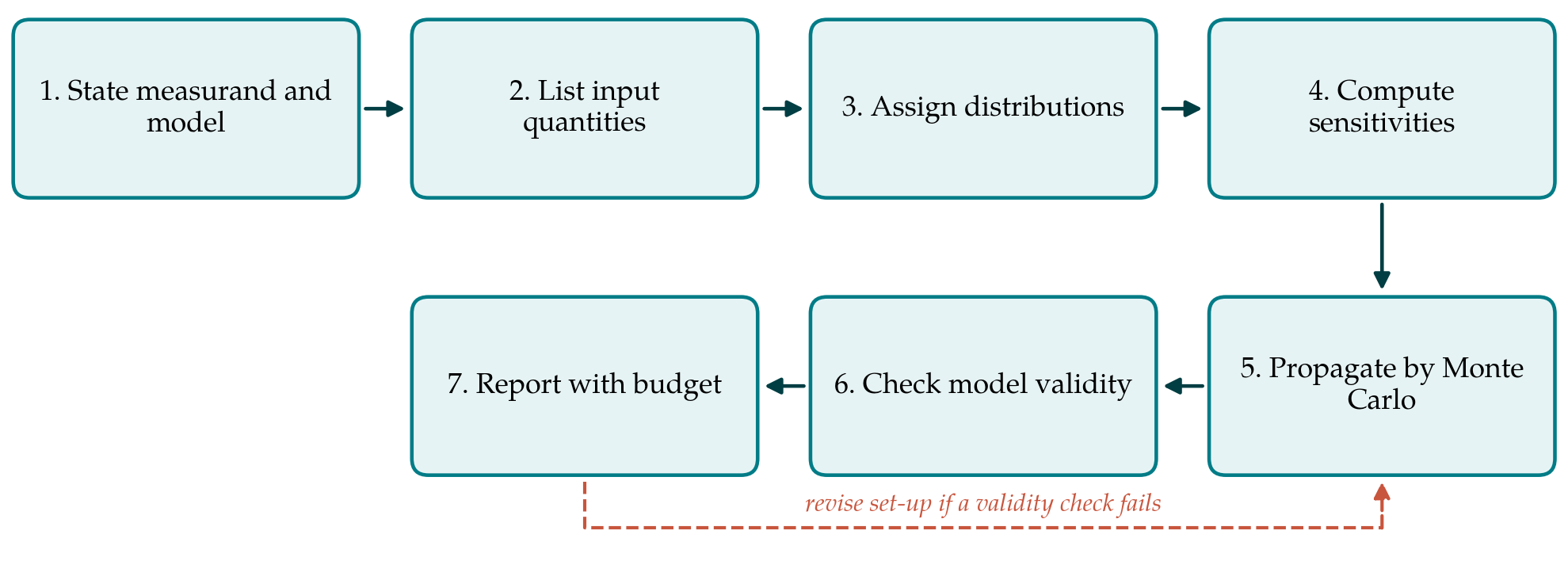
3.1. Step 1: State the measurand and the model
The statement begins by saying what is being measured: for example, the thermal conductivity of a named material at a stated mean temperature, in a stated direction if the material is anisotropic, at a stated moisture condition if it is porous. The evaluation model is then written down in full, including the sensor geometry, the form of D(τ), the fitted parameters and the criterion by which the time window is chosen. Writing it out exposes which quantities are inputs with their own uncertainty and which are outputs of the fit.
3.2. Step 2: List the input quantities
Every quantity that enters the model, or that could make the experiment depart from it, is listed. Table 1 gives a starting list. Some inputs are instrumental and the same for every test with a given sensor. Others belong to the specimen and its mounting and change from test to test.
3.3. Step 3: Assign a distribution to each input
Each input receives a probability distribution. Where repeated observations exist, such as the noise of the temperature signal, a normal distribution with the observed standard deviation is appropriate. Where only limits are known, such as a tolerance on radius, the GUM recommends a rectangular distribution between the limits. Calibration certificates supply a standard uncertainty directly. The reasons for each assignment are recorded, because a reader can only judge the final figure by judging these choices. Correlations should be noted: the temperature coefficient and the power both depend on the same resistance measurement.
3.4. Step 4: Compute sensitivity coefficients
Before any propagation, each input is perturbed by a small amount and the evaluation is rerun on the recorded transient to find the change in conductivity. The resulting sensitivity coefficients show which inputs matter, and they can differ sharply from one material to another. They also reveal the condition of the fit. Parameter estimation theory shows that two parameters cannot be separated if their sensitivity curves are proportional over the time window (Beck and Arnold, 1977), and a near-proportionality between the sensitivities to conductivity and diffusivity is a warning that the window is poorly chosen. Where inputs interact strongly, a variance-based global analysis is more informative than one-at-a-time perturbation (Saltelli et al., 2008).
3.5. Step 5: Propagate the distributions
Values of all inputs are drawn from their distributions, the full evaluation, including the iteration and the fit, is repeated for each draw, and the resulting conductivities are collected. Supplement 1 gives guidance on the number of trials and on extracting a coverage interval from the output distribution (JCGM, 2008b). Noise in the transient is included by resampling the residuals of the fit or by adding synthetic noise of the observed variance. The linear GUM combination, using the coefficients from Step 4, should be computed alongside. Agreement between the two gives confidence in both, and disagreement shows that the model is too nonlinear for the simpler method.
3.6. Step 6: Check the validity of the model
Propagation only covers uncertainty within the model. Whether the model fits the experiment is a separate question, and three checks address it. The probing depth, conventionally taken as 2(αt)1/2 at the end of the window, must be smaller than the distance from the sensor edge to the nearest specimen boundary. The residuals of the fit should scatter randomly about zero; a systematic curve indicates boundary effects, contact resistance or drift. And the whole procedure should be run on a reference material of similar conductivity. If a check fails, the set-up is changed and the measurement repeated; a larger uncertainty is not a substitute.
The third check matters most for insulating materials. Zheng et al. (2020) showed that the standard evaluation can overestimate the conductivity of low-conductivity specimens because the sensor and its insulating film store and conduct a non-negligible share of the heat, which the ideal model ignores. A bias of this kind has to be corrected, or included as a separate component with its own justification.
3.7. Step 7: Report
The result is reported as a value with an expanded uncertainty and a stated coverage probability, together with the conditions of Step 1, the sensor, the power, the measurement time and the window used. The uncertainty budget, giving each input, its distribution, its sensitivity and its contribution, should accompany the result or be available on request, as laboratories working to recognised quality systems already do. Reporting the fitted diffusivity with its own uncertainty costs nothing extra and lets a reader test the result for consistency against an independent heat capacity.
4. Fitting the Procedure to Practice
The effort required depends on access to the raw transient. Commercial software exports the recorded temperature rise, and the evaluation described in the standard can be reproduced in a short script, after which Steps 4 and 5 are automatic. A laboratory need not repeat the full analysis for every specimen. A reasonable practice is to carry it out once for each class of material and sensor, keep the resulting budget as a template, and rerun only the checks of Step 6 and the specimen-dependent inputs for routine tests. The published assessment of the transient hot-wire method by Hammerschmidt and Sabuga (2000) is a useful model of what a complete budget for a transient technique looks like.
Some materials need special attention. For anisotropic specimens the heat capacity input usually dominates the budget. For moist or porous materials the measurand of Step 1 must fix the moisture state, since heating can redistribute moisture during the test. For liquids the measurement time has to be short enough to avoid convection, and its onset is a validity check in the sense of Step 6.
5. Limitations and What Remains to Be Shown
The procedure is a proposal. It has not been tested here on measured transients, and three questions would need answers before it could be recommended as standard practice. The first is whether the intervals it produces are realistic: on certified reference materials, the reference value should fall within the stated interval about as often as the coverage probability implies. The second is whether different laboratories applying the procedure to the same material arrive at compatible budgets, which only an interlaboratory comparison can show. The third is how sensitive the outcome is to the Type B judgements of Step 3, in particular the treatment of contact and of the sensor's own heat capacity.
There are also limits of principle. Monte Carlo propagation cannot reveal an effect that is absent from the model, so the checks of Step 6 carry real weight and depend on the availability of reference materials in the relevant conductivity range. Material inhomogeneity is a property of the specimen and not an uncertainty of the measurement, and it should be reported separately as the spread between specimens.
6. Conclusion
A transient plane source result is the output of a fit, and its uncertainty cannot be read from an instrument specification. The seven-step procedure proposed here treats the evaluation as a measurement model in the sense of the GUM, identifies the inputs that carry uncertainty, propagates them numerically through the complete fitting routine, and separates that calculation from checks on whether the ideal model applies. It asks for more work than quoting a nominal accuracy, mainly at the first use for a new class of material. Whether it yields intervals that hold up against reference materials and between laboratories remains to be demonstrated.
Conflict of interest
To be declared by the author(s) before publication.
Funding
To be declared by the author(s) before publication.