International Journal of Nuclear Science and Technology

Uncertainty Quantification Steps for Thermal Hydraulic System Codes in Safety Analysis

Seojun Tanaka¹, Minjun Iyer², Lerato Espinoza³

¹ Department of Science, Andes School of Science, Switzerland, ² Department of Science, Dalmatian University Centre for Science, United Kingdom, ³ Department of Science, Zambezi Institute of Science, Cote d'Ivoire

Published 12 Jun 2026 Vol. 1, Article 3 10.62715/ijnst.2026.v1.i1.pp15-20 0 accesses 0 citations

Download PDF XML HTML EPUB

0Accesses

0Citations

Abstract

Best estimate plus uncertainty analysis has become an accepted way of demonstrating that a nuclear power plant meets its acceptance criteria in design basis accidents. It replaces deliberately pessimistic models with realistic ones and requires in exchange a quantified statement of how uncertain the calculated result is. The underlying methods, from the Code Scaling, Applicability and Uncertainty evaluation methodology to the order-statistics approach associated with Wilks' formula, are well documented, but they are described in separate places, at different levels of detail, and an analyst new to the subject has to assemble a working sequence from them. This article proposes such a sequence in eight steps: fix the scenario and figures of merit, rank the phenomena, confirm that the code and nodalisation are applicable, characterise the input uncertainties, plan the sample and propagate, screen the calculations, derive tolerance limits and compare them with the criteria, and carry out sensitivity analysis and reporting. For each step the article states the purpose, the decisions the analyst must take and justify, and the common errors. The procedure is assembled from published methods and regulatory guidance. It is a proposal that has not been applied or validated in this article, and the closing sections state what it does not resolve.

Keywords: Sensitivity analysis Best estimate plus uncertainty Thermal hydraulics System codes Wilks formula Safety analysis

1. Introduction

Thermal hydraulic system codes such as RELAP5, TRACE, CATHARE and ATHLET calculate how a reactor coolant system behaves during transients and loss-of-coolant accidents. Their results are compared with acceptance criteria, of which the limit on peak cladding temperature in emergency core cooling analysis is the best known. For many years the comparison was made with conservative evaluation models, in which pessimistic assumptions were prescribed so that the calculated result would bound reality without the margin being known. Regulatory practice now also admits realistic calculations, on condition that their uncertainty is evaluated and accounted for when the result is compared with the limit (USNRC, 1989; IAEA, 2019).

The methods for doing so matured over three decades. The Code Scaling, Applicability and Uncertainty (CSAU) evaluation methodology gave the subject its structure (Boyack et al., 1990). The method developed at Gesellschaft für Anlagen- und Reaktorsicherheit (GRS) made statistical propagation practical by using order statistics, so that the number of code runs does not grow with the number of uncertain inputs (Glaeser, 2008). International comparison exercises then showed how much the outcome depends on choices made by the analyst (OECD-NEA, 2011).

An engineer who must carry out such an analysis for the first time finds the necessary guidance spread across regulatory guides, safety reports and journal papers. This article gathers it into one ordered procedure. The procedure is proposed as a working aid. It is not applied to a plant or an experiment here, no results are reported, and it has not been validated as a whole.

2. Background

The uncertainty of a system code result has several origins. The closure relations for interfacial friction, wall heat transfer, critical flow and similar processes are empirical and were fitted to experiments of limited range. The plant is represented by a nodalisation that averages over three-dimensional detail. Initial and boundary conditions, material properties and equipment performance are known only within tolerances. Numerical solution adds its own error, and the user's modelling decisions add more. Oberkampf and Roy (2010) distinguish aleatory uncertainty, which reflects inherent variability, from epistemic uncertainty, which reflects lack of knowledge. In system code analysis most contributors are epistemic, although they are commonly described by probability distributions for the purpose of propagation.

Two families of method are in use (IAEA, 2008). The first propagates input uncertainties: ranges and distributions are assigned to uncertain inputs, the code is run many times with sampled values, and the spread of the output is analysed. CSAU and the GRS method belong here. The second extrapolates output uncertainty: the differences between calculation and measurement in a database of integral experiments are processed and carried over to the plant calculation, as in the methodology based on accuracy extrapolation of D'Auria et al. (1995). The procedure proposed below follows the first family, which is the more widely used, while drawing on the second for its insistence on qualified nodalisations.

The statistical core of the propagation approach is the result of Wilks (1941) on distribution-free tolerance limits. If N independent runs are made with randomly sampled inputs, the largest output is an upper bound on the 95th percentile with confidence 1 − 0.95N, whatever the form of the output distribution. A confidence of 95% is first reached with 59 runs, which is the origin of the figure quoted throughout the field. Wald (1943) extended the result to several outputs considered jointly.

3. The Proposed Procedure

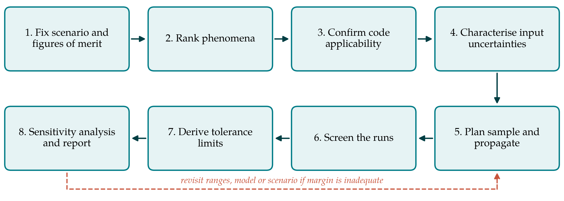
The procedure has eight steps, listed in Table 1 with the product each should deliver. Figure 1 shows their order and the return path that applies when the result leaves insufficient margin. The steps reorganise the elements of CSAU and of the evaluation model development process in regulatory guidance (USNRC, 2005) around the decisions an analyst takes in practice.

Table 1: Steps of the proposed procedure, the main decision at each step and the product it delivers
Step	Main decision	Product
1. Scenario and figures of merit	Which transient, plant state and acceptance criteria are addressed	Analysis specification
2. Phenomena ranking	Which processes most affect each figure of merit in each phase	Phenomena identification and ranking table
3. Code applicability	Whether code, version and nodalisation are qualified for those processes	Assessment matrix and frozen input model
4. Input uncertainties	Which inputs are uncertain, with what ranges and distributions	Justified list of uncertain parameters
5. Sampling and propagation	Sample size, order of tolerance limit and sampling scheme	Sampling plan and completed runs
6. Screening	How failed or unphysical runs are treated	Run log with dispositions
7. Tolerance limits	How the limit is derived and compared with the criterion	Statement of result with coverage and confidence
8. Sensitivity and reporting	Which inputs drive the spread and how the work is recorded	Sensitivity measures and final report

Figure 1: Sequence of the eight proposed steps, with the return path used when the calculated margin is inadequate

3.1. Step 1: Fix the scenario and the figures of merit

An uncertainty analysis is specific to a plant, a transient and a set of output quantities. The analyst states the initiating event, the assumed plant state and single failure, and the figures of merit with their acceptance criteria. Scalar quantities such as a peak temperature or a minimum collapsed level are simpler to treat than time-dependent ones. If several criteria must be met simultaneously, this has to be declared now, because it changes the sample size required in Step 5.

3.2. Step 2: Identify and rank the phenomena

The transient is divided into phases, and for each phase the phenomena that could influence the figures of merit are listed and ranked by a panel with access to experimental evidence. The resulting phenomena identification and ranking table directs effort to what matters and provides the justification for leaving low-ranked items at nominal values (Wilson and Boyack, 1998). The ranking is a judgement, and should be recorded with its reasons and revisited when the sensitivity results of Step 8 are available.

3.3. Step 3: Confirm code applicability and freeze the model

For each highly ranked phenomenon the analyst shows that the code has been assessed against separate-effect and integral tests covering the relevant conditions, and that scale distortion between tests and plant has been considered. The plant nodalisation should follow the practices used in the assessment calculations, since a nodalisation tuned to one test does not carry its qualification elsewhere. Code version, options and input model are then frozen. Changing them after the uncertainty runs have begun invalidates the sample.

3.4. Step 4: Characterise the input uncertainties

Each uncertain input receives a range and a probability distribution with a recorded basis: scatter of the data behind a correlation, comparison of the code with separate-effect tests, manufacturing tolerances, technical specification limits or, where nothing better exists, expert judgement. Experience from the BEMUSE programme identified this step as the largest source of difference between participants who used the same code on the same problem (OECD-NEA, 2011). Model parameters, for which no direct measurement exists, are the hardest case. Inverse methods that infer their distributions from experimental data are an active research area (Wu et al., 2018) and can supplement judgement where suitable data exist. Known dependencies between inputs should be represented, and a uniform distribution should not be mistaken for a neutral choice.

3.5. Step 5: Plan the sample and propagate

The sample size follows from the coverage and confidence required, the order of the tolerance limit and the number of outputs treated jointly. For a one-sided 95%/95% statement on a single output the first-order limit needs 59 runs. Taking the second or third largest value as the limit requires 93 or 124 runs respectively and gives a less scattered estimate. Guba et al. (2003) set out the corresponding requirements when several outputs must satisfy their limits together, and Nutt and Wallis (2004) discuss the alternatives. This procedure recommends planning for more than the minimum, both to reduce the conservatism of the first-order limit and to leave room for failed runs.

Inputs are drawn by simple random sampling, which is the assumption under which Wilks' formula holds. Latin hypercube sampling (McKay et al., 1979) covers the input space more evenly and is attractive for sensitivity work, but its samples are not independent in the sense the formula requires, so it should not be combined with the order-statistics limit without separate justification. The seed and the sampled values are archived so that the set can be regenerated.

3.6. Step 6: Screen the calculations

Every run is checked for completion, mass and energy balance, and physically reasonable behaviour. Runs that fail for numerical reasons present a statistical difficulty, because discarding them silently biases the sample if failure is correlated with severe conditions. The defensible options are to repair and rerun the case with the same sampled inputs, or to treat failed runs as if they had exceeded the highest valid result and raise the order of the tolerance limit accordingly. Whichever is chosen, the rule is set before the results are seen.

3.7. Step 7: Derive tolerance limits and compare with the criteria

The outputs are ranked and the value of the planned order is taken as the tolerance limit. The result is stated in full: for example, that with at least 95% confidence, at least 95% of the output population lies below the stated value, given the input distributions assumed. The qualifying clause matters. The statement is conditional on Step 4 and says nothing about contributors that were not sampled. The limit is then compared with the acceptance criterion. If the margin is inadequate, the legitimate responses are to improve the knowledge behind the dominant input ranges, to refine the model, or to change the plant or scenario assumptions. Repeating the sample until a favourable set appears is not among them.

3.8. Step 8: Sensitivity analysis and reporting

The same runs support a first sensitivity analysis. Rank correlation coefficients between each input and each output indicate which inputs drive the spread, with the caution that at sample sizes near one hundred only the strongest influences are distinguishable from chance. Variance-based indices give a fuller picture but need far more evaluations, usually through a surrogate model (Saltelli et al., 2008). The findings are compared with the ranking of Step 2, and disagreements are investigated. The report records every step in enough detail for an independent analyst to repeat the work.

4. Fitting the Procedure to Practice

The effort is unevenly distributed. Steps 2 to 4 consume most of the time on a first application and little on later ones for the same plant and code, since the ranking table, the assessment basis and the parameter list can be reused with revision. Steps 5 to 7 are largely automated once scripts for sampling, job submission and post-processing exist. An organisation adopting the procedure should therefore expect a high initial cost and treat the documented basis for input uncertainties as an asset to be maintained.

The procedure also needs adjusting to the regulatory setting. Some regulators expect the acceptance criterion to be met at 95% probability with 95% confidence; others accept different formulations or ask for additional deterministic conservatisms on selected inputs such as decay heat or the availability of safety systems (IAEA, 2019). These requirements enter at Step 1 and should be settled with the regulator before calculations begin.

5. Limitations and What Remains to Be Shown

The procedure is a synthesis and has not been tested here. Its usefulness would have to be shown by applying it to an integral experiment for which measurements are available, so that the calculated uncertainty band can be compared with data, and then by independent teams applying it to the same plant problem to see whether it narrows the spread between analysts. Until that is done it should be read as a structured checklist grounded in published methods and not as a qualified methodology.

Some difficulties lie outside its reach. Order statistics control sampling uncertainty and nothing else; they do not compensate for an input range that is too narrow or a phenomenon the code does not model. Nodalisation and user effects are held fixed, not quantified. Scenarios with threshold behaviour, in which a small input change switches the transient onto a different path, can produce output distributions whose upper tail is poorly sampled by a hundred runs. Finally, the meaning of a probability statement built on epistemic input distributions continues to be debated in the regulatory literature (Nutt and Wallis, 2004).

6. Conclusion

Uncertainty quantification for system code calculations rests on methods that are individually well established. What the practitioner needs is their arrangement into a sequence with the decisions made explicit. The eight steps proposed here provide one such arrangement, with emphasis on justifying input uncertainties, fixing statistical rules in advance and stating results with their conditions. The procedure awaits demonstration on experimental and plant cases, and it is offered as a basis for that work.

Conflict of interest

To be declared by the author(s) before publication.

Funding

To be declared by the author(s) before publication.

References

[1] Boyack, B.E., Catton, I., Duffey, R.B., Griffith, P., Katsma, K.R., Lellouche, G.S., Levy, S., Rohatgi, U.S., Wilson, G.E., Wulff, W. and Zuber, N. Quantifying reactor safety margins Part 1: An overview of the code scaling, applicability, and uncertainty evaluation methodology. Nuclear Engineering and Design https://doi.org/10.1016/0029-5493(90)90071-5 119(1), 1-15 (1990).
[2] D'Auria, F., Debrecin, N. and Galassi, G.M. Outline of the uncertainty methodology based on accuracy extrapolation. Nuclear Technology 109(1), 21-38 (1995).
[3] Glaeser, H. GRS method for uncertainty and sensitivity evaluation of code results and applications. Science and Technology of Nuclear Installations https://doi.org/10.1155/2008/798901 2008, 798901 (2008).
[4] Guba, A., Makai, M. and Pál, L. Statistical aspects of best estimate method-I. Reliability Engineering & System Safety 80(3), 217-232 (2003).
[5] IAEA Best Estimate Safety Analysis for Nuclear Power Plants: Uncertainty Evaluation. Safety Reports Series No. 52. International Atomic Energy Agency, Vienna (2008).
[6] IAEA Deterministic Safety Analysis for Nuclear Power Plants. IAEA Safety Standards Series No. SSG-2 (Rev. 1). International Atomic Energy Agency, Vienna (2019).
[7] McKay, M.D., Beckman, R.J. and Conover, W.J. A comparison of three methods for selecting values of input variables in the analysis of output from a computer code. Technometrics 21(2), 239-245 (1979).
[8] Nutt, W.T. and Wallis, G.B. Evaluation of nuclear safety from the outputs of computer codes in the presence of uncertainties. Reliability Engineering & System Safety 83(1), 57-77 (2004).
[9] Oberkampf, W.L. and Roy, C.J. Verification and Validation in Scientific Computing. Cambridge University Press, Cambridge (2010).
[10] OECD-NEA BEMUSE Phase VI Report: Status Report on the Area, Classification of the Methods, Conclusions and Recommendations. NEA/CSNI/R(2011)4. OECD Nuclear Energy Agency, Paris (2011).
[11] Saltelli, A., Ratto, M., Andres, T., Campolongo, F., Cariboni, J., Gatelli, D., Saisana, M. and Tarantola, S. Global Sensitivity Analysis: The Primer. John Wiley & Sons, Chichester (2008).
[12] USNRC Best-Estimate Calculations of Emergency Core Cooling System Performance. Regulatory Guide 1.157. U.S. Nuclear Regulatory Commission, Washington, DC (1989).
[13] USNRC Transient and Accident Analysis Methods. Regulatory Guide 1.203. U.S. Nuclear Regulatory Commission, Washington, DC (2005).
[14] Wald, A. An extension of Wilks' method for setting tolerance limits. Annals of Mathematical Statistics 14(1), 45-55 (1943).
[15] Wilks, S.S. Determination of sample sizes for setting tolerance limits. Annals of Mathematical Statistics https://doi.org/10.1214/aoms/1177731788 12(1), 91-96 (1941).
[16] Wilson, G.E. and Boyack, B.E. The role of the PIRT process in experiments, code development and code applications associated with reactor safety analysis. Nuclear Engineering and Design 186(1-2), 23-37 (1998).
[17] Wu, X., Kozlowski, T., Meidani, H. and Shirvan, K. Inverse uncertainty quantification using the modular Bayesian approach based on Gaussian process, Part 1: Theory. Nuclear Engineering and Design 335, 339-355 (2018).

Article metrics

0 total accesses since publication. 0 citing articles have been indexed to date.