1. Introduction
A capacitive soil moisture sensor does not measure water. It measures how readily an oscillating electric field charges the soil around its electrodes, a property that depends mainly on the dielectric permittivity of the soil, and it relies on the large contrast between the permittivity of liquid water, about 80 at room temperature, and that of mineral grains and air. The principle has been in use for decades, and the access-tube probes and low-cost pronged sensors built on it have made continuous records of soil water routine (Robinson et al., 2008).
The conversion from sensor output to water content is empirical. For time domain reflectometry a single equation serves a wide range of mineral soils (Topp et al., 1980), and manufacturers of capacitive sensors supply comparable general equations. Comparative tests show that such standard functions perform acceptably in sands and loams and progressively worse as clay content and salinity rise (Vaz et al., 2013). Heavy clays, among them the Vertisols on which much irrigated cotton, sorghum and rice is grown, are the soils in which a general equation is least trustworthy and in which water management matters a great deal.
This article sets out a procedure for calibrating capacitive sensors in such soils against gravimetric sampling. It is written for irrigation engineers and agronomists who have an oven, a balance and a set of core rings but no dielectric laboratory. The procedure is proposed on the basis of the published literature. No calibration data are reported, and the claims made for it are limited to its logic.
2. Why Heavy Clays Defeat General Equations
Four properties of clay soils disturb the relation between permittivity and water content, and a fifth disturbs the reference measurement itself.
2.1. Bound water, conductivity and frequency
Clay minerals, smectites above all, have a very large specific surface, and the first layers of water adsorbed on it are not free to rotate with the field. Their permittivity is far below that of bulk water, so a given sensor reading corresponds to more water in a clay than in a sand (Saarenketo, 1998). Clays also conduct electricity through their exchangeable cations. At the frequencies used by capacitive sensors, which are commonly well below those of time domain reflectometry, conduction and interfacial polarisation add to the apparent permittivity, and the effect grows as frequency falls (Robinson et al., 2003). Laboratory work on a widely used low-cost sensor found its response to electrical conductivity and temperature to be small at its operating frequency of 70 MHz (Kizito et al., 2008), but sensors that run at lower frequencies are less well protected, and an independent evaluation of a sensor of this class reported measurable effects of temperature, conductivity and supply voltage (Bogena et al., 2007).
Temperature acts in two directions. The permittivity of free water falls as it warms, while bound water is released from surfaces and conductivity rises, so the net temperature response of a clay can be positive where that of a sand is negative (Wraith and Or, 1999). A sensor at shallow depth therefore shows a daily wave that is not a change in water content. An evaluation of a 50 MHz sensor likewise found that its response differed between soils, most of all in those rich in clay, which points to soil-specific calibration (Seyfried and Murdock, 2004).
2.2. Shrinkage, cracks and the moving reference
A swelling clay changes volume as it dries. Over much of the range the loss of volume nearly equals the volume of water lost, the soil surface subsides, and cracks open (Bronswijk, 1988). Two consequences follow. A crack or a thin air gap beside an electrode lowers the reading sharply, because the sensor is most sensitive to the material closest to it. And the dry bulk density of the soil matrix rises as water content falls, so the conversion from gravimetric to volumetric water content, which multiplies by bulk density, cannot use a single value measured once (Grossman and Reinsch, 2002). A calibration for a clay must determine volume and mass on the same sample every time.
3. The Proposed Procedure
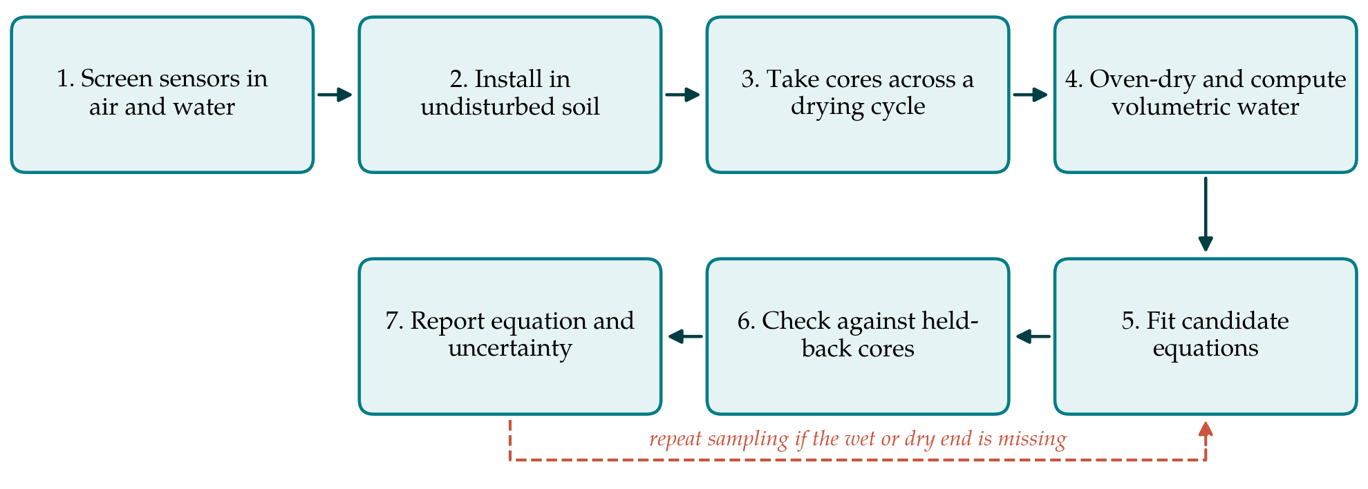
The procedure calibrates the sensors where they will be used, in soil that has not been dried, sieved and repacked. Repacking is convenient and gives a wide range of water contents quickly, but it destroys the structure and the shrinkage behaviour that make the clay difficult, and comparative work on the accuracy of profiling sensors has relied on field calibration against volumetric samples for that reason (Evett et al., 2006). Figure 1 shows the sequence of steps. Table 1 lists the sources of error peculiar to heavy clay and the point in the procedure at which each is addressed.
| Source of error | Effect on the calibration | Response in the procedure |
|---|---|---|
| Bound water and dispersion | General equation misreads water content (Saarenketo, 1998) | Soil-specific equation fitted to field cores (Step 5) |
| Changing bulk density | Volumetric reference biased if one density is assumed | Volume and mass measured on every core (Steps 3 and 4) |
| Cracks and air gaps | Low and erratic readings in dry soil | Moist installation; cracks recorded; core between cracks (Steps 2 and 3) |
| Temperature | Daily wave unrelated to water content | Fixed sampling hour; temperature logged and tested as a term |
| Sensor-to-sensor spread | One equation does not fit all units | Screening in air and water (Step 1) |
| Spatial variability | Core and sensor see different soil | Replicate cores close to replicate sensors (Step 3) |
3.1. Step 1: Screen the sensors
Sensors of one model do not respond identically. Before installation each sensor is read in air and in water at a recorded temperature, and where possible in one or two liquids of intermediate permittivity, following the approach used to quantify sensor-to-sensor variability (Rosenbaum et al., 2010). Sensors whose readings fall well outside the group are set aside. The spread of the remainder is kept, because it sets a floor under the uncertainty of any calibration that will be applied to sensors other than those calibrated.
3.2. Step 2: Install in undisturbed soil
Installation is done when the soil is moist and plastic, so that the prongs can be pressed into the wall of a small pit or the base of an auger hole without leaving a gap. At least three sensors are placed at each depth of interest, far enough apart for cores to be taken between them later. A soil temperature sensor is installed at the same depth. The pit is backfilled in layers to its original density, and the site is left through one wetting event before sampling starts, so that the soil closes around the sensors.
3.3. Step 3: Sample across a full drying cycle
The calibration is only as wide as the range of water contents sampled. The plot is wetted to saturation by ponding, then allowed to dry under the crop or under a rain shelter, and cores are taken on six to ten occasions spread from the wettest to the driest condition the sensors will meet. On each occasion two or three cores are cut with thin-walled rings of known volume at the depth of the sensors and within a short horizontal distance of them, in the manner laid down for volumetric sampling (ISO, 2001). The sensor output and the soil temperature are logged at the moment of sampling, and the readings are taken at the same hour each time to limit the diurnal temperature effect. When cracks have formed, cores are taken from the intact soil between cracks, and the presence and width of cracks near the sensors are noted.
3.4. Step 4: Determine the reference water content
Each core is sealed in the field, weighed moist, dried in a ventilated oven at 105 °C until its mass is constant, and weighed again. Gravimetric water content is the mass of water lost divided by the oven-dry mass, bulk density is the oven-dry mass divided by the ring volume, and volumetric water content is their product divided by the density of water (Gardner, 1986). Because the ring fixes the volume at the moment of sampling, the bulk density obtained is the one that applied at that water content. Smectitic clays retain some structural water at 105 °C and take a long time to reach constant mass. The convention is kept nonetheless, so that results are comparable with other work, and the drying time actually needed is established on a few trial cores.
3.5. Step 5: Fit candidate equations
The paired values of sensor output and volumetric water content are plotted before anything is fitted. Three forms are then compared: a straight line in raw output, a second-order polynomial, and a line in the square root of apparent permittivity where the sensor reports it, which corresponds to the refractive index mixing model and has been used to calibrate a common capacitive sensor in sands from two reference points (Sakaki et al., 2008). Soil temperature is tested as an additional term and retained only if it clearly reduces the residual scatter. The simplest equation whose residuals show no trend with water content is preferred. Higher-order polynomials are avoided, since they behave unpredictably at the ends of the range, which are the conditions that trigger irrigation decisions.
3.6. Step 6: Check against held-back cores
A calibration judged on the data used to fit it looks better than it is. Before fitting, the cores from one or two sampling occasions near the middle of the range, or from one of the replicate sensors, are set aside. The fitted equation is applied to these and the differences between predicted and gravimetric values are summarised by their mean, which estimates bias, and by the root mean square error. A plot of each difference against the mean of the two values, with limits of agreement, shows whether the error depends on wetness (Bland and Altman, 1986). The same statistics are computed for the manufacturer's equation, so that the gain from calibrating is stated and not assumed.
3.7. Step 7: Report
The report gives the soil classification, clay content and mineralogy if known, the sensor model and firmware, the range of water content and temperature covered, the bulk density at each sampling, the equation with the standard errors of its coefficients, and the validation statistics. The uncertainty of the reference itself, which combines the tolerances of the ring volume and the balance with the scatter between replicate cores, is stated following the conventions of the international guide (JCGM, 2008). An equation is not to be used outside the range of water contents over which it was fitted, and the report says so.
4. Fitting the Procedure to Practice
The work is modest in equipment and heavy in visits. A drying cycle in a clay under a crop may last several weeks, and the sampler must return on each occasion with rings, a mallet, sealed tins and the logger. Where a full cycle cannot be followed, the two ends matter most: one sampling shortly after drainage has slowed and one at the driest state expected. Coring removes soil, so the plot must be large enough for all samples to come from undisturbed ground, and each hole is refilled and marked. On farms with several distinct clay soils, a separate calibration is needed for each, and it is prudent to check the equation with a few cores in the following season, since cracking patterns and contact with the electrodes change after a full cycle of shrinking and swelling.
5. Limitations and What Remains to Be Shown
The procedure has been reasoned out from the literature and has not been tried here. Its central assumption is that a core taken a short distance from a sensor represents the soil the sensor responds to. Capacitive sensors sample a small volume close to their electrodes, much smaller than a core, and in a structured clay the two may differ systematically. Whether replicate cores overcome this is an empirical matter. It is also unsettled how far an equation obtained at one depth and one season can be carried to others, how large the temperature term is in a given clay, and whether the dry end of the range, where cracks dominate, can be calibrated at all with sensors of this kind. A first application should report these points directly, including the cases in which the calibrated sensor still disagrees with the oven.
6. Conclusion
General calibration equations for capacitive sensors rest on soils unlike heavy clays, and the physical reasons for their failure in clays are understood. The procedure proposed in this article answers each of those reasons with a specific step, and it treats bulk density as a quantity to be measured at every sampling. It requires patience more than apparatus. Its accuracy in practice, and the limits of its transfer between sites and seasons, are for field application to establish.
Conflict of interest
To be declared by the author(s) before publication.
Funding
To be declared by the author(s) before publication.