1. Introduction
Soil organic carbon varies over distances of metres. Old field boundaries, erosion and deposition along slopes, patches of different drainage and decades of uneven manure application all leave their mark, and a single composite sample per field averages them away. A farmer who wants to manage that variation, or a project that must demonstrate a change in carbon stock against it, needs many more observations than a laboratory budget ordinarily allows. Reviews of soil carbon monitoring identify the cost of measurement as the main obstacle to credible verification (Smith et al., 2020).
Diffuse reflectance spectroscopy in the visible and near-infrared range, from 350 to 2500 nm, offers a way round the constraint. The spectrum of a soil sample carries information on organic matter, clay minerals, iron oxides and water, and multivariate calibration can extract estimates of several properties from one scan (Viscarra Rossel et al., 2006; Stenberg et al., 2010). The idea is not new: Ben-Dor and Banin (1995) demonstrated simultaneous prediction of several soil properties from near-infrared spectra three decades ago. What has changed is that rugged portable spectrometers now make it practical to scan soil where it lies.
Published studies describe the pieces of a field method in detail, but they are scattered across the literatures of chemometrics, soil spectroscopy and digital soil mapping. This article assembles them into one workflow suited to a single farm. The workflow is a proposal. No field trial is reported, and the article is explicit about what a trial would have to show.
2. Background
Organic matter darkens soil across the visible range and produces weak, overlapping absorptions in the near-infrared that arise from overtones and combinations of the fundamental vibrations of C-H, N-H and O-H bonds. None of these features is sharp enough to be read off directly, which is why calibration against reference measurements is always required (Stenberg et al., 2010). Large spectral libraries have been built to supply such calibrations at regional and global scale (Viscarra Rossel et al., 2016), and a critical review of the technique for carbon stock assessment concluded that its accuracy depends heavily on how closely the calibration samples resemble the soils to be predicted (Bellon-Maurel and McBratney, 2011).
Field spectra differ from laboratory spectra of dried, sieved soil. Water absorbs strongly near 1400 and 1900 nm and lowers reflectance across the whole range, while surface roughness, aggregates and stray light add further variation unrelated to carbon. Two families of correction exist. External parameter orthogonalisation removes from the spectra the directions of variation that moisture induces (Minasny et al., 2011). Direct standardisation transforms field spectra so that they resemble their laboratory counterparts (Ji et al., 2015). Either allows a calibration built on dry spectra to be applied in the field.
3. The Proposed Workflow
The workflow has six stages. Table 1 lists them with the principal decision at each and the record that should be kept, and the subsections that follow take them in order.
| Stage | Principal decision | Record kept |
|---|---|---|
| 1. Stratify and locate | Covariates used; number of scan locations | Covariate layers, coordinates of locations |
| 2. Acquire spectra | Surface or core; replicate scans; reference panel interval | Scan log, instrument settings, soil condition |
| 3. Reference subset | Size of subset; selection rule | Sample list, laboratory method and report |
| 4. Preprocess | Smoothing, scatter and moisture correction | Processing script and parameters |
| 5. Calibrate and validate | Model type; local, spiked or library calibration | Validation statistics on independent samples |
| 6. Map | Interpolation method; covariates | Prediction and uncertainty maps |
3.1. Stage 1: Stratify the farm and choose scan locations
Scan locations should span the variation in the factors that control carbon, not merely the geographic extent of the farm. Digital soil mapping provides the framework: soil properties are predicted from spatially exhaustive covariates representing terrain, parent material, vegetation and management (McBratney et al., 2003). For a farm the covariates might be a digital elevation model and its derivatives, bare-soil satellite imagery, yield maps and field boundaries. Conditioned Latin hypercube sampling selects locations that reproduce the joint distribution of the covariates with a set number of points (Minasny and McBratney, 2006). Because a scan is cheap, the number of locations can be several times what conventional sampling would afford.
3.2. Stage 2: Acquire spectra to a fixed protocol
Consistency matters more than any particular choice. The protocol should fix whether spectra are taken on a scraped surface, on the wall of a small pit or on an extracted core; the use of a contact probe with its own light source, which excludes ambient light; the number of replicate scans per location, each on a fresh face; and the interval at which a white reference panel is read. Stones, residue and roots are cleared from the measured face. The instrument is allowed to warm up before the first reading, and a small set of check samples kept in sealed containers is scanned at the start and end of each day so that drift can be detected and, if necessary, corrected. The operator notes the moisture condition of the soil, and where depth increments are wanted a core is scanned at set depths. Every location is georeferenced.
3.3. Stage 3: Select a subset for reference analysis
Only a fraction of the scanned locations is sampled for the laboratory. The fraction should be chosen from the spectra themselves, so that the calibration set covers the spectral diversity of the farm. The algorithm of Kennard and Stone (1969) does this by picking samples that are successively furthest from those already chosen. Samples are dried, sieved and analysed for organic carbon by dry combustion with correction for carbonates, the method standardised as ISO 10694 (1995). Wet oxidation with dichromate, the Walkley-Black procedure, is cheaper and still widely used, but it recovers only part of the organic carbon and requires a correction factor that varies between soils, which adds uncertainty to a calibration built on it. The dried samples are also scanned, to provide the paired dry and field spectra that the moisture correction requires.
3.4. Stage 4: Preprocess and correct the spectra
Raw reflectance is first trimmed of the noisy ends of the range and of any detector splice artefacts, and replicate scans are averaged. Standard treatments follow. Smoothing and differentiation with the filter of Savitzky and Golay (1964) suppress noise and baseline shifts, and the standard normal variate transformation reduces multiplicative scatter effects caused by particle size and surface texture (Barnes et al., 1989). The moisture correction is then derived from the paired spectra of Stage 3 and applied to all field spectra. Every parameter belongs in a script, so that the processing can be repeated exactly when the farm is resurveyed.
3.5. Stage 5: Calibrate and validate
Partial least squares regression remains the reference method for spectral calibration (Wold et al., 2001), and it is a sensible default for the few dozen samples a farm calibration is likely to have. Three calibration strategies are open. A purely local model uses only the farm's own samples. A library model uses an existing regional library and no local samples, and usually predicts poorly at a new site. Spiking adds a small number of local samples to a library subset and often recovers most of the accuracy of a local model at lower cost (Guerrero et al., 2010). Whichever is chosen, accuracy must be judged on samples that took no part in model fitting or tuning. The root mean square error and bias of those predictions should be reported in the units of the measurement; ratio statistics alone are a weak guide, as Bellon-Maurel et al. (2010) explain.
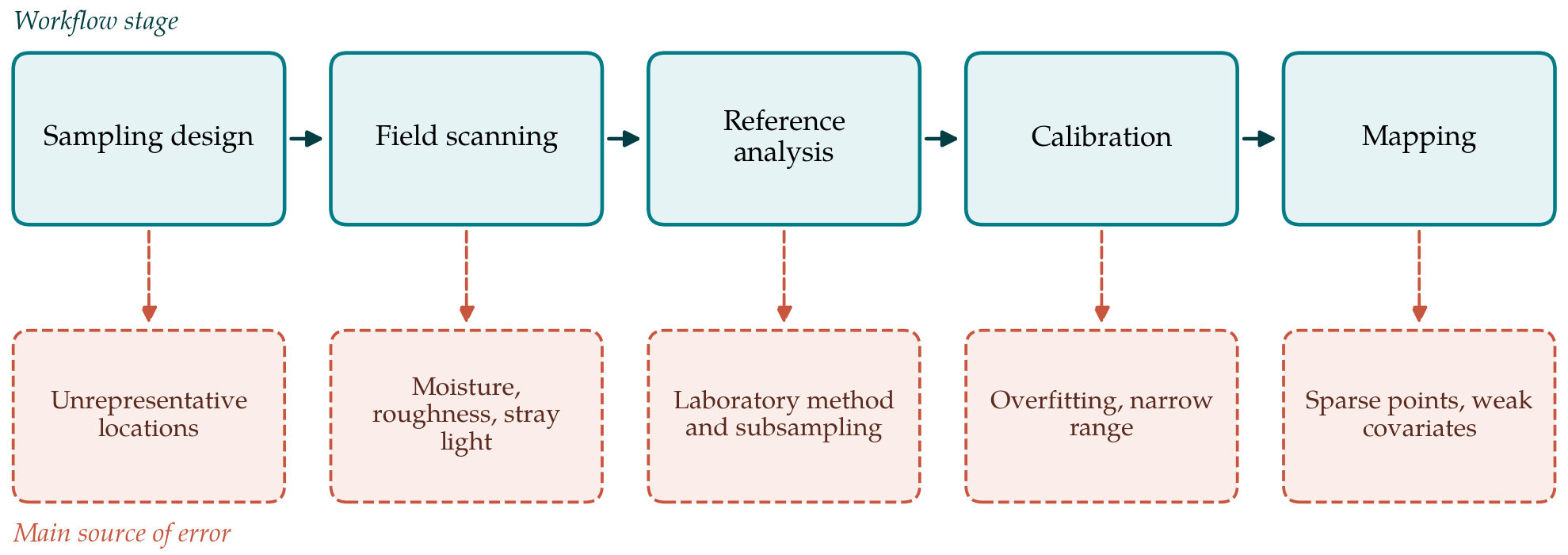
Figure 1 pairs each stage of the workflow with the source of error that most threatens it. The validation error estimated at this stage includes the errors of scanning and reference analysis, but it does not include the error of interpolation, which arises only at the next stage.
3.6. Stage 6: Map the predictions and their uncertainty
The calibrated model converts every field spectrum to a carbon estimate, giving a dense set of points. A continuous surface is obtained by kriging or, where covariates explain part of the pattern, by regression kriging, in which a trend fitted to the covariates is combined with kriging of the residuals (McBratney et al., 2003). The variogram should be inspected for adequate numbers of point pairs at short lags, following the guidance of Webster and Oliver (2007). The prediction variance from kriging understates the true uncertainty because the points themselves carry calibration error. The two should be combined, at the least by adding the validation error variance from Stage 5, and the uncertainty map delivered alongside the carbon map.
4. Fitting the Workflow to a Farm
The economics of the method rest on the ratio of scans to laboratory samples. Scanning is quick once the operator is practised, and the laboratory cost is confined to the calibration subset and a validation set. A resurvey some years later can reuse the calibration if a small set of new reference samples confirms that it still holds, which is where the method offers most to monitoring. The instrument is the main capital cost, and for a single farm sharing through an advisory service or cooperative is more realistic than purchase.
Timing affects quality. Scanning is best done when the soil is neither saturated nor baked hard, and when the surface is free of a growing crop. A map of carbon concentration is also not a map of carbon stock. Stock requires bulk density and the content of coarse fragments for each depth increment, and the spectrometer measures neither reliably. Those must come from core sampling at a subset of locations.
5. Limitations and What Remains to Be Shown
This article has proposed a workflow without applying it, and several of its assumptions need testing. The first is that a moisture correction derived from a modest number of paired spectra is stable across the range of field conditions met during a survey. The second is that a calibration subset chosen by spectral diversity is large enough to give a trustworthy independent validation, given that samples withheld for validation reduce those available for fitting. The third concerns range: on a farm where carbon varies little, the calibration error may be comparable to the variation to be mapped, and the map will then show mostly noise.
For carbon accounting the requirement is stricter still. Detecting a change in stock between two surveys demands that the combined error of both be small relative to the change, and that bias be constant between them. Whether field spectroscopy meets that standard at farm scale is an open question in the literature. Sandy soils low in carbon, soils with carbonates and soils rich in iron oxides are known to be difficult cases for visible and near-infrared calibrations.
6. Conclusion
Portable spectrometers make it feasible to observe soil organic carbon at a density that laboratory analysis alone cannot reach. The workflow proposed here arranges established techniques, covariate-based sampling, protocol-driven scanning, spectrally guided reference sampling, moisture correction, independently validated calibration and geostatistical mapping, into a sequence a practitioner can follow and document. It is offered for trial. The decisive evidence will be independent validation at the level of the final map, on farms of contrasting soils, with the full error budget reported.
Conflict of interest
To be declared by the author(s) before publication.
Funding
To be declared by the author(s) before publication.