International Journal of VLSI Designing and Signal Processing

Approximate Multiplier Architectures for Energy-Constrained Image Processing Accelerators in Edge Devices: A Review of Design Approaches

Selam Okonkwo¹, Ananya Balogun², Precious Lee³

¹ Department of Electrical Electronics, Rhone Research Institute of Electrical Electronics, Croatia, ² Department of Electrical Electronics, Lapland Institute for Advanced Electrical Electronics, Colombia, ³ Department of Electrical Electronics, Bharathapuzha Institute for Advanced Electrical Electronics, Ethiopia

Published 11 Jul 2026 Vol. 1, Article 1 10.62715/ijvlsidsp.2026.v1.i1.pp1-7 0 accesses 0 citations

Download PDF XML HTML EPUB

0Accesses

0Citations

Abstract

Multiplication dominates the arithmetic cost of the filters, transforms and convolutional layers that make up most image processing pipelines, and on battery-powered edge devices that cost is paid in energy. Because the output of such pipelines is judged by human viewers or by classifiers that tolerate noise, a multiplier need not return the exact product every time. This narrative review surveys the published architectures that exploit this freedom. It groups them by the place in the multiplier where the approximation is introduced: the generation of partial products, their reduction by compressor or adder trees, the reduction of the operands themselves through truncation, segmentation or logarithmic encoding, and automated methods that search for inexact circuits under a quality constraint. For each family the review describes the mechanism, the character of the error it produces, and the conditions under which it suits image workloads. It then examines the error metrics used to compare designs and how poorly some of them predict perceived image quality, and considers what changes when a multiplier is embedded in a complete accelerator. The review closes with open problems, including verification, runtime accuracy control and the limited evidence at system level.

Keywords: Approximate computing Approximate multipliers Image processing Edge accelerators Energy-efficient arithmetic Error metrics

1. Introduction

A camera node that sharpens, compresses or classifies its own images performs millions of multiplications per frame. Convolution kernels, the discrete cosine transform, colour space conversion and the layers of a neural network all reduce to multiply-accumulate operations, and a multiplier costs far more energy than an adder of the same word length. Horowitz (2014) set out why this matters: with supply voltage scaling largely exhausted, further gains in computing efficiency have to come from specialisation and from doing less work per result. For a device that runs from a small battery or from harvested energy, the arithmetic datapath is one of the few places left where a designer can still remove work.

Approximate computing removes work by relaxing the requirement that a circuit be numerically exact. The idea rests on the observation that many applications are error resilient: their inputs are noisy, their outputs are consumed by human senses or statistical models, and there is no single correct answer (Han and Orshansky, 2013). Surveys of the area cover techniques at every level from programming languages to transistors (Mittal, 2016). Within that broad field, inexact arithmetic units have attracted the most sustained attention from circuit designers, and the multiplier, being large and regular, offers the most room for savings.

This review concentrates on one question: which approximate multiplier architectures are suited to image processing accelerators in edge devices, and what is known about how to choose among them. It describes the main design families, the error behaviour each produces, the measures by which designs are compared, and the issues that arise when a multiplier is placed inside a full datapath. It reports no new measurements. Its purpose is to organise a scattered literature for the designer who has to make the choice.

2. Scope and Approach

The article is a narrative review of the published literature on approximate integer and fixed-point multipliers, drawing on the main circuit design, computer arithmetic and design automation venues and on two earlier comparative surveys (Jiang et al., 2017; Jiang et al., 2020). Sources were selected because they introduced an architecture that later work built on, or because they connect arithmetic error to image quality. Voltage overscaling, in which an exact circuit is run below its safe supply voltage, and stochastic computing are outside the scope, as are floating-point units. No claim of exhaustive coverage is made, and figures reported by individual papers are not restated, since they were obtained on different technologies and with different tools and cannot fairly be set side by side.

3. Why Image Workloads Tolerate Inexact Products

Three properties of image processing explain its tolerance. Pixel data are quantised to a small number of bits and already carry sensor noise, so an error in the low-order bits of a product is often below the noise floor. Most kernels accumulate many products, and if the errors are of mixed sign and small mean they partly cancel in the sum. Finally, the result is normally rounded, clipped and requantised before it is displayed or passed on, which discards much of the precision that an exact multiplier would have preserved. Gupta et al. (2013) used image and video compression to show that inexact adders in the transform datapath can leave the decoded picture visually acceptable, and the same argument carries over to multipliers.

Tolerance is not uniform across a pipeline. An error that is harmless in a smoothing filter may be amplified in an edge detector, where differences of nearly equal quantities are taken, and errors introduced early in a transform can spread across a whole block. Neural networks for vision add a further case. Their weights are learned, the network can be retrained with the inexact multiplier in the loop, and the designs that work best are those whose error is small for the operand values that occur most often (Mrazek et al., 2016). The practical consequence is that a multiplier cannot be judged in isolation from the kernel it serves.

4. Architectural Families

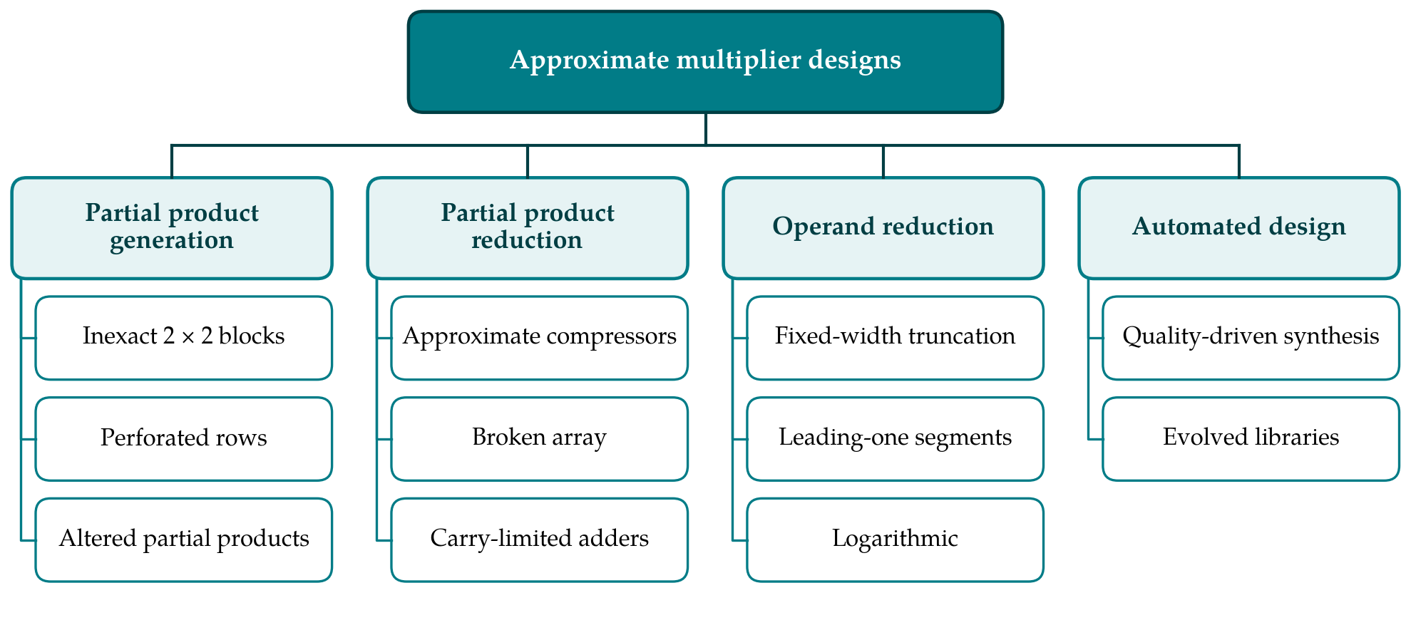
An unsigned array or tree multiplier works in three stages. It forms partial products, either by AND gates or by Booth recoding of one operand (Booth, 1951). It reduces them to two rows with a tree of counters or compressors, following the schemes of Wallace (1964) and Dadda (1965). It then adds the two rows in a carry-propagate adder. Approximation can be introduced in any stage or applied to the operands before the multiplier is reached. Figure 1 arranges the published designs by that point of entry, and Table 1 summarises the families discussed in the subsections that follow.

Table 1: Families of approximate multiplier and their suitability for image processing datapaths
Family	Mechanism	Character of the error	Representative sources
Inexact building blocks	Small multiplier block with a simplified truth table	Bounded; occurs for specific operand patterns	Kulkarni et al., 2011
Perforation and altered partial products	Rows omitted or recombined before reduction	Analytically bounded; one-sided for perforation	Zervakis et al., 2016; Venkatachalam and Ko, 2017
Approximate reduction	Inexact compressors or pruned adder cells in low-order columns	Small magnitude, frequent	Momeni et al., 2015; Mahdiani et al., 2010
Fixed-width truncation	Low-order columns dropped, constant added	Small absolute error, nearly unbiased	Schulte and Swartzlander, 1993
Dynamic or static segments	Short operand segments multiplied exactly, then shifted	Bounded relative error, near-zero mean	Hashemi et al., 2015; Narayanamoorthy et al., 2015
Logarithmic	Add approximate logarithms, convert back	Relative error of one sign unless corrected	Mitchell, 1962
Automated search	Synthesis or evolution under an error constraint	Chosen by the constraint; no closed form	Mrazek et al., 2017

Figure 1: Classification of approximate multiplier designs by the stage at which inexactness is introduced

4.1. Approximation in partial product generation

Kulkarni et al. (2011) proposed building a multiplier from 2 × 2 blocks in which a single entry of the truth table is wrong: the product of three and three is returned as seven, which fits in three bits and so removes logic from every block. Larger multipliers are assembled from these blocks with exact adders, and the error is bounded and occurs only for particular operand patterns. A second route is partial product perforation, in which whole rows of the partial product matrix are omitted (Zervakis et al., 2016). Perforation is easy to apply to an existing design and the error can be expressed in closed form, which helps when a quality bound has to be guaranteed. Venkatachalam and Ko (2017) instead transform the partial products into generate and propagate terms and apply inexact adders and compressors only to the less significant columns.

4.2. Approximation in partial product reduction

The reduction tree holds most of the gates, so it has been the most frequent target. The 4-2 compressor is the standard cell of fast reduction trees, and Momeni et al. (2015) presented two simplified versions that give wrong outputs for a few input combinations, then studied where in a Dadda tree they may be used. Their analysis established a point that later work has repeated: inexact cells belong in the low-order columns, and exact cells must be kept where the weight is high. The broken-array multiplier of Mahdiani et al. (2010) removes carry-save adder cells below a chosen diagonal of an array multiplier, giving a family of designs indexed by how much of the array is cut away.

Liu et al. (2014) took a different line. Their multiplier accumulates partial products with an adder whose carry propagation is deliberately limited, which shortens the critical path, and it generates an error signal that can be added back for a configurable number of the most significant bits. The recovery width becomes a design parameter that trades accuracy against delay and power.

4.3. Truncation, segmentation and logarithmic schemes

The oldest form of approximate multiplication predates the term. A fixed-width multiplier discards the least significant columns of the partial product matrix and adds a constant to compensate for the mean of what was dropped (Schulte and Swartzlander, 1993). The error is small in absolute terms and biased only slightly, and the method remains the baseline against which newer designs should be compared. Segmentation methods shrink the operands instead of the matrix. The dynamic range unbiased multiplier of Hashemi et al. (2015) finds the leading one of each operand, keeps a short segment starting there, sets the lowest retained bit to one so that the error has near-zero mean, multiplies the segments in a small exact core and shifts the result. The static segment method of Narayanamoorthy et al. (2015) chooses among a few fixed segment positions, which avoids the leading-one detector and barrel shifter at some cost in accuracy.

Segment-based designs bound the relative error, not the absolute error, and this suits data with a wide dynamic range. Logarithmic multipliers share the property. Following Mitchell (1962), they approximate the binary logarithm of each operand by a piecewise linear function, add the logarithms and convert back, so that multiplication is replaced by shifting and addition. The error of the basic scheme is always of one sign, and much later work consists of correction terms that reduce it.

4.4. Automated and library-based design

Hand-designed architectures explore a small part of the space of inexact circuits. Automated approximation treats the problem as synthesis under a quality constraint. SALSA encodes the constraint as a function of the outputs and uses the resulting don't-care conditions to simplify the logic (Venkataramani et al., 2012). Evolutionary methods search over gate-level netlists directly: the EvoApprox8b library offers several hundred eight-bit multipliers and adders spread along the trade-off between error and power, each obtained by Cartesian genetic programming (Mrazek et al., 2017). Such libraries let a designer pick a circuit by its measured error statistics without knowing its structure. The price is that the circuits are irregular, hard to scale to other word lengths and offer no analytical error bound.

5. Error Metrics and Image Quality

Arithmetic papers characterise a design by statistics taken over all operand pairs. The error rate is the fraction of inputs for which the output is wrong. The error distance is the absolute difference between the exact and the approximate product, and its mean, often normalised by the largest possible output, is the most widely reported single figure (Liang et al., 2013). The mean relative error distance divides each error by the exact result. Worst-case error and bias, the signed mean of the error, complete the usual set. These quantities are convenient because they are properties of the circuit alone, and the comparative studies of Jiang et al. (2017) rely on them.

Their weakness is the assumption of uniformly distributed operands. Pixel values, filter coefficients and network weights are far from uniform: coefficients are often small or zero, and activations cluster near zero after rectification. A multiplier with an unimpressive mean error distance may be almost exact over the operand range a kernel uses, and the reverse can also hold. Bias deserves particular attention in accumulating datapaths, since a one-sided error grows with the number of terms summed while a zero-mean error grows only with its square root.

At application level, quality is usually reported as peak signal-to-noise ratio against the output of an exact pipeline, or as the structural similarity index of Wang et al. (2004), which was designed to follow perceived quality more closely than pixel-wise error does. For classification workloads the measure is the change in accuracy. None of these can be derived from the arithmetic metrics in general. The relation depends on the kernel, the image content and the position of the multiplier in the pipeline, which is why careful studies evaluate each candidate inside the target application.

6. From Multiplier to Accelerator

Savings reported for a stand-alone multiplier shrink once it is embedded. In an accelerator the multipliers share the energy budget with memories, line buffers, control logic and clock distribution, and for neural network accelerators the movement of data between memory and datapath is frequently the larger cost (Sze et al., 2017). An inexact multiplier therefore has to be weighed against simpler measures that also cut arithmetic energy, above all a shorter word length. A fair comparison sets each approximate design against an exact multiplier of reduced precision that delivers the same output quality, a baseline that is not always included.

Several accelerator-level techniques make better use of a given inexact design. Where coefficients are constants, as in a fixed filter or a trained network, the designer can choose for each multiplier position the cheapest circuit that is accurate for that coefficient. Where quality requirements change at run time, for instance between a preview mode and a capture mode, a design with a configurable error recovery stage or selectable perforation allows accuracy to be exchanged for energy without a second datapath. On gate arrays the picture differs again, because multiplication is mapped to look-up tables, carry chains and hard blocks, and gate-level simplifications conceived for standard cells do not carry over without redesign.

7. Gaps and Directions for Future Work

The first gap is comparability. Designs are synthesised on different cell libraries, at different timing constraints and with different test images, so their reported gains cannot be ranked. Open libraries of circuits with published error data are a partial remedy, and shared benchmark pipelines with agreed quality thresholds would be another. The second is verification. An exact multiplier has one specification; an approximate one needs a formal statement of its permitted error and a method for proving that the implementation respects it at every word length used. Simulation over all inputs is feasible at eight bits and impractical well before thirty-two.

A third gap concerns signed and Booth-encoded multipliers, which practical datapaths use but which much of the literature sets aside in favour of unsigned arrays. A fourth is the interaction with other sources of inexactness in the same pipeline, such as quantised weights, lossy compression and sensor noise: whether errors from several sources add, mask one another or compound has rarely been examined. Finally, most evidence comes from synthesis estimates. Silicon measurements of complete image pipelines built with approximate multipliers remain scarce, and until more are published the size of the benefit at system level is uncertain.

8. Conclusion

The published architectures for approximate multiplication fall into a small number of families, distinguished by where the inexactness enters and by the kind of error that results. For image processing at the edge, the error profile matters more than the headline energy figure: designs with small, zero-mean error suit accumulating kernels, designs with bounded relative error suit data of wide dynamic range, and any candidate should be compared with a plain reduction in word length. The arithmetic metrics in common use are a first filter and no more. The choice has to be confirmed inside the intended pipeline, with its real operand statistics and a quality measure that reflects how the images will be used.

Conflict of interest

To be declared by the author(s) before publication.

Funding

To be declared by the author(s) before publication.

References

[1] Booth, A.D. A signed binary multiplication technique. The Quarterly Journal of Mechanics and Applied Mathematics https://doi.org/10.1093/qjmam/4.2.236 4(2), 236-240 (1951).
[2] Dadda, L. Some schemes for parallel multipliers. Alta Frequenza 34, 349-356 (1965).
[3] Gupta, V., Mohapatra, D., Raghunathan, A. and Roy, K. Low-power digital signal processing using approximate adders. IEEE Transactions on Computer-Aided Design of Integrated Circuits and Systems https://doi.org/10.1109/TCAD.2012.2217962 32(1), 124-137 (2013).
[4] Han, J. and Orshansky, M. Approximate computing: An emerging paradigm for energy-efficient design. Proceedings of the 18th IEEE European Test Symposium https://doi.org/10.1109/ETS.2013.6569370 (2013).
[5] Hashemi, S., Bahar, R.I. and Reda, S. DRUM: A dynamic range unbiased multiplier for approximate applications. Proceedings of the IEEE/ACM International Conference on Computer-Aided Design https://doi.org/10.1109/ICCAD.2015.7372600 418-425 (2015).
[6] Horowitz, M. Computing's energy problem (and what we can do about it). IEEE International Solid-State Circuits Conference Digest of Technical Papers https://doi.org/10.1109/ISSCC.2014.6757323 10-14 (2014).
[7] Jiang, H., Liu, C., Liu, L., Lombardi, F. and Han, J. A review, classification, and comparative evaluation of approximate arithmetic circuits. ACM Journal on Emerging Technologies in Computing Systems https://doi.org/10.1145/3094124 13(4), 60 (2017).
[8] Jiang, H., Santiago, F.J.H., Mo, H., Liu, L. and Han, J. Approximate arithmetic circuits: A survey, characterization, and recent applications. Proceedings of the IEEE https://doi.org/10.1109/JPROC.2020.3006451 108(12), 2108-2135 (2020).
[9] Kulkarni, P., Gupta, P. and Ercegovac, M. Trading accuracy for power with an underdesigned multiplier architecture. Proceedings of the 24th International Conference on VLSI Design https://doi.org/10.1109/VLSID.2011.51 346-351 (2011).
[10] Liang, J., Han, J. and Lombardi, F. New metrics for the reliability of approximate and probabilistic adders. IEEE Transactions on Computers https://doi.org/10.1109/TC.2012.146 62(9), 1760-1771 (2013).
[11] Liu, C., Han, J. and Lombardi, F. A low-power, high-performance approximate multiplier with configurable partial error recovery. Proceedings of the Design, Automation and Test in Europe Conference and Exhibition (2014).
[12] Mahdiani, H.R., Ahmadi, A., Fakhraie, S.M. and Lucas, C. Bio-inspired imprecise computational blocks for efficient VLSI implementation of soft-computing applications. IEEE Transactions on Circuits and Systems I: Regular Papers https://doi.org/10.1109/TCSI.2009.2027626 57(4), 850-862 (2010).
[13] Mitchell, J.N. Computer multiplication and division using binary logarithms. IRE Transactions on Electronic Computers https://doi.org/10.1109/TEC.1962.5219391 EC-11(4), 512-517 (1962).
[14] Mittal, S. A survey of techniques for approximate computing. ACM Computing Surveys https://doi.org/10.1145/2893356 48(4), 62 (2016).
[15] Momeni, A., Han, J., Montuschi, P. and Lombardi, F. Design and analysis of approximate compressors for multiplication. IEEE Transactions on Computers https://doi.org/10.1109/TC.2014.2308214 64(4), 984-994 (2015).
[16] Mrazek, V., Hrbacek, R., Vasicek, Z. and Sekanina, L. EvoApprox8b: Library of approximate adders and multipliers for circuit design and benchmarking of approximation methods. Proceedings of the Design, Automation and Test in Europe Conference and Exhibition https://doi.org/10.23919/DATE.2017.7926993 258-261 (2017).
[17] Mrazek, V., Sarwar, S.S., Sekanina, L., Vasicek, Z. and Roy, K. Design of power-efficient approximate multipliers for approximate artificial neural networks. Proceedings of the 35th International Conference on Computer-Aided Design https://doi.org/10.1145/2966986.2967021 (2016).
[18] Narayanamoorthy, S., Moghaddam, H.A., Liu, Z., Park, T. and Kim, N.S. Energy-efficient approximate multiplication for digital signal processing and classification applications. IEEE Transactions on Very Large Scale Integration (VLSI) Systems https://doi.org/10.1109/TVLSI.2014.2333366 23(6), 1180-1184 (2015).
[19] Schulte, M.J. and Swartzlander, E.E. Truncated multiplication with correction constant. Proceedings of the IEEE Workshop on VLSI Signal Processing VI 388-396 (1993).
[20] Sze, V., Chen, Y.-H., Yang, T.-J. and Emer, J.S. Efficient processing of deep neural networks: A tutorial and survey. Proceedings of the IEEE https://doi.org/10.1109/JPROC.2017.2761740 105(12), 2295-2329 (2017).
[21] Venkatachalam, S. and Ko, S.-B. Design of power and area efficient approximate multipliers. IEEE Transactions on Very Large Scale Integration (VLSI) Systems https://doi.org/10.1109/TVLSI.2016.2643639 25(5), 1782-1786 (2017).
[22] Venkataramani, S., Sabne, A., Kozhikkottu, V., Roy, K. and Raghunathan, A. SALSA: Systematic logic synthesis of approximate circuits. Proceedings of the 49th Annual Design Automation Conference https://doi.org/10.1145/2228360.2228504 796-801 (2012).
[23] Wallace, C.S. A suggestion for a fast multiplier. IEEE Transactions on Electronic Computers https://doi.org/10.1109/PGEC.1964.263830 EC-13(1), 14-17 (1964).
[24] Wang, Z., Bovik, A.C., Sheikh, H.R. and Simoncelli, E.P. Image quality assessment: From error visibility to structural similarity. IEEE Transactions on Image Processing https://doi.org/10.1109/TIP.2003.819861 13(4), 600-612 (2004).
[25] Zervakis, G., Tsoumanis, K., Xydis, S., Soudris, D. and Pekmestzi, K. Design-efficient approximate multiplication circuits through partial product perforation. IEEE Transactions on Very Large Scale Integration (VLSI) Systems https://doi.org/10.1109/TVLSI.2016.2535398 24(10), 3105-3117 (2016).

Article metrics

0 total accesses since publication. 0 citing articles have been indexed to date.