1. Introduction
A municipal treatment works typically meters raw water at the inlet, treated water at the outlet and a number of internal streams such as filter backwash and chemical carrier water. The outlet meter carries particular weight. It is the system input volume in the water balance from which leakage and other losses are estimated (Lambert et al., 1999), so an error there propagates directly into every loss figure the utility reports. Audit guidance for water utilities accordingly treats verification of production meters as an early and essential task of a water audit (AWWA, 2016).
Suspicion usually begins with a mismatch. The inlet and outlet totals disagree by more than the known internal uses, the reservoir fed by the works fills faster or slower than the metered inflow implies, or pump energy per unit volume shifts without explanation. The meter is checked, perhaps exchanged, and the mismatch remains. An error that outlasts the obvious remedy is what this article calls persistent. The reference texts on flow measurement devote at least as much space to installation effects and secondary instrumentation as to the primary element (Baker, 2016), and it is in those areas, together with configuration and data handling, that a persistent error is most plausibly sought.
The article proposes a procedure for diagnosing such errors in an orderly way. It is written for the instrument engineer or technician at a utility, with full-bore electromagnetic meters chiefly in mind because they dominate closed-pipe measurement at treatment works, and with notes on other meter types. The procedure is put forward for trial. It is not a report of an investigation at any plant, and no plant data are presented.
2. Background
The electromagnetic flowmeter applies Faraday's law to a conducting liquid: a magnetic field across the pipe induces between two wall electrodes a voltage proportional to the mean velocity. The theory was set out by Shercliff (1962), and Bevir (1970) showed through the weight-function concept how the contribution of each part of the cross-section to the signal depends on the field design, which explains why a distorted velocity profile shifts the reading. The meter has no moving parts, causes no head loss and holds its calibration well, which is why a persistent error in one is seldom a matter of simple wear. Current guidance on selection, installation and use is given in an international standard (ISO, 2017) and in the water-industry manual on flowmeters (AWWA, 2006).
Other meter types found at treatment works bring their own sensitivities. Differential-pressure devices such as Venturi tubes depend on geometry, tapping condition and the transmitter that reads them (ISO, 2003; Miller, 1996). Transit-time ultrasonic meters depend on the assumed pipe dimensions and on profile (Lynnworth and Liu, 2006). Flumes and weirs on open channels convert a level to a flow through a rating that holds only if the approach conditions and the downstream level are as assumed (Bos, 1989). The sensitivity of flowmeters to upstream fittings such as elbows was documented in the tests of Mattingly and Yeh (1991).
Two ideas from metrology frame the procedure. A discrepancy between two measurements is meaningful only in relation to their combined uncertainty (JCGM, 2008), and the uncertainty of a flow measurement includes installation and secondary instrumentation as well as the calibration of the primary device (ISO, 2005). A meter that meets its accuracy class on a calibration rig, as defined for water meters in the metrological standards (OIML, 2013; ISO, 2014), can still deliver a wrong total to the control room.
3. The Proposed Procedure
The procedure has eight steps, shown in Figure 1. They are ordered so that inexpensive checks that need no access to the pipe come first, and so that each step narrows the field for the next. A step is not skipped because its fault seems unlikely, since the premise of a persistent error is that the likely cause has already been tried.
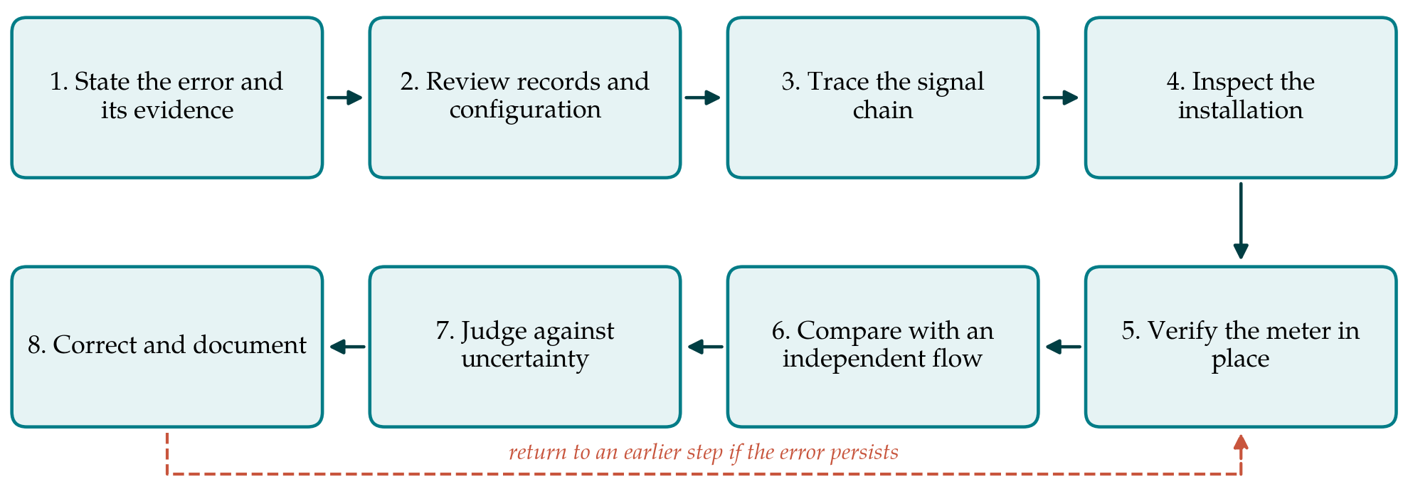
3.1. Step 1: State the error and its evidence
The investigator writes down what is believed to be wrong, by how much, in which direction, since when, and on what evidence. The evidence is nearly always a comparison, so the comparison is examined as critically as the meter. A mass balance across the works needs every stream that crosses the boundary, including backwash, sludge, sampling and overflow, and needs the change in storage over the balance period. Plotting the difference against time and against flow rate is the most informative single act of the whole procedure, because the pattern of the error points to its class, as Table 1 indicates.
| Pattern observed | Causes to consider first | Step that tests them |
|---|---|---|
| Constant offset, present at zero flow | Zero drift, earthing fault, low-flow cut-off disabled, loop current offset | Steps 3 and 5 |
| Constant percentage at all flows | Wrong calibration factor, range or pulse scaling; wrong pipe diameter entered | Steps 2 and 3 |
| Error changes with flow rate | Distorted velocity profile, partly full pipe, meter outside its range | Step 4 |
| Error appeared on a known date | Configuration change, replaced component, altered pipework or valve position | Step 2 |
| Intermittent or noisy | Entrained air, electrode coating, electrical interference, loose connection | Steps 4 and 5 |
| Totals disagree, instantaneous rates agree | Totaliser scaling, missed pulses, data gaps, time-base mismatch | Step 3 |
| Slow growth over months | Deposits reducing the bore, liner deformation, drift of a pressure transmitter | Steps 4 and 5 |
3.2. Step 2: Review records and configuration
The calibration certificate, the nameplate and the parameters stored in the converter are compared line by line. The calibration factor in the converter must be the one on the certificate for that serial number, a point that is easily lost when electronics are exchanged between sensors. The nominal diameter, the full-scale value, the pulse weight, the damping time, the low-flow cut-off and the flow direction are recorded. The sizing of the meter is checked against the actual operating range, since a meter chosen for the ultimate design flow of the works may spend its life at the bottom of its range, where the relative error permitted by its class is larger. The maintenance log is read for anything that coincides with the onset of the discrepancy.
3.3. Step 3: Trace the signal chain
The reported figure passes through several conversions between the converter and the monthly return. The current output is scaled to engineering units at an input card; the range entered there must match the range in the converter. A known current is injected at the transmitter terminals and the value followed to the operator display and the historian. Where volume is totalised from pulses, the pulse weight and the maximum pulse frequency of the receiving input are checked, and where it is integrated from the rate signal, the integration interval, the treatment of missing samples and the handling of signals below the cut-off are examined. The converter's own totaliser is read at the start and end of a period and compared with the reported total for the same period. A disagreement here closes the investigation of the primary device before it has begun.
3.4. Step 4: Inspect the installation
The installation is compared with what the manufacturer and the standard require (ISO, 2017). The straight lengths upstream and downstream are measured and the nearest fittings identified, with particular attention to partly open valves, bends in two planes and pumps close upstream, all of which produce asymmetric or swirling profiles (Mattingly and Yeh, 1991). The pipe must run full at the meter. A meter at a high point, on a descending leg or immediately before a free discharge may be partly empty or carry air at low flows, and an electromagnetic meter interprets the whole bore as liquid. Chemical injection points just upstream can create local conductivity variations and noise. The earthing arrangement is checked against the drawing, as are grounding rings on lined or non-metallic pipe, the routing of signal cable and the integrity of cable glands.
3.5. Step 5: Verify the meter in place
Most current electromagnetic meters can be checked in place with a verification tool, built in or connected externally, that tests coil resistance and inductance, electrode circuit impedance, insulation and the linearity and zero of the converter against values recorded at the factory. A pass shows that the magnetic circuit and electronics have not changed, which is strong evidence that the calibration factor still applies. It is not a flow calibration. It cannot see a change in the bore caused by deposits or a deformed liner, and it says nothing about the velocity profile. Where the meter can be isolated full of still water, the zero is read directly. If the works can spare the line, the sensor is removed and the bore and electrodes inspected and measured. For a differential-pressure meter the equivalent step is a check of the transmitter against a pressure standard and inspection of the tappings and impulse lines.
3.6. Step 6: Compare with an independent flow
If the earlier steps find nothing, the meter is compared with a second measurement that shares none of its components. Three options are generally available at a treatment works, in increasing order of effort. A clamp-on transit-time ultrasonic meter (Lynnworth and Liu, 2006) can be fitted on a suitable straight length; its result depends on accurate pipe diameter, wall thickness and lining data, and its uncertainty is usually several times that of the meter under test, so it detects gross error only. A volumetric test uses a clear-water tank or service reservoir of surveyed dimensions as a measuring vessel, timing the change of level with all other connections isolated, in the manner of the volumetric-tank method used on calibration rigs (ISO, 1987). An insertion probe or a tracer dilution test gives a further independent value where a tapping exists. Whatever the method, the comparison is made at several flow rates that span the operating range.
3.7. Step 7: Judge the difference against uncertainty
An uncertainty budget is written for both the plant meter and the reference, with contributions for calibration, installation effects, secondary instrumentation, tank dimensions and level reading, and timing, combined in the usual way (JCGM, 2008; ISO, 2005). If the difference lies within the expanded uncertainty of the comparison, the test has not demonstrated an error, and the original evidence of Step 1 should be re-examined. If it lies outside, the size and flow dependence of the difference are compared with the patterns of Table 1 and the investigation returns to the step indicated.
3.8. Step 8: Correct and document
The remedy follows from the cause: reconfiguration, repair of earthing, relocation of the meter or of a dosing point, fitting of a flow conditioner, cleaning, or replacement with a meter of suitable size. After the change, Step 6 is repeated to confirm the result. The file records the initial evidence, each check with its finding, including those that found nothing, the uncertainty budget and the final comparison. A cause-and-effect diagram of the kind long used in quality control is a convenient summary and a useful aid for the next investigation.
4. Fitting the Procedure to a Working Plant
A treatment works cannot usually stop to suit an investigation. Steps 1 to 3 need no interruption and can be completed within days from the office and the control room. Step 4 is a walk-down with drawings. Step 5 needs a permit and, for a zero check, brief isolation. Step 6 is the one that requires planning with operations, since a reservoir drop test ties up storage and must be scheduled for a period of low demand. Utilities with several works will find it economical to hold one clamp-on meter and one verification tool centrally and to train a small team in their use and their limits. The management of production meters then becomes part of a wider programme of meter management of the kind described for customer meters by Arregui et al. (2006).
5. Limitations and What Remains to Be Shown
The procedure has not been applied to a plant in the course of this work, and its usefulness is untested. A trial would need to establish at least two things: whether the ordering of steps finds causes with less effort than the unstructured practice it is meant to replace, and whether the patterns in Table 1 discriminate between causes as cleanly in real records as they do in principle, given that plants often suffer more than one fault at once. The table is a guide to where to look first and not a decision rule.
The independent comparison of Step 6 is the weakest link. Field reference methods rarely achieve an uncertainty better than that claimed for a well-installed electromagnetic meter, so small errors of the order of the meter's own class cannot be confirmed on site and may only be resolved by removal to a calibration laboratory. Large-diameter meters are costly to remove and few laboratories can test them. The procedure therefore resolves gross and moderate errors with more confidence than fine ones, and that boundary should be stated in any report that uses it.
6. Conclusion
A flowmeter error that persists after the meter has been checked is a sign that the fault lies in the measurement system around the meter, or in the evidence that first raised the alarm. The eight-step procedure proposed here directs attention accordingly: to the statement of the discrepancy, the configuration, the signal chain and the installation before the primary device, and to an explicit comparison of any residual difference with its uncertainty. It asks for no equipment that a utility of moderate size does not already own or cannot borrow. Its merit will be settled by use, and documentation of each investigation in the form proposed would, over time, supply the evidence.
Conflict of interest
To be declared by the author(s) before publication.
Funding
To be declared by the author(s) before publication.