1. Introduction
A batch reactor is run to a recipe, and the recipe is written in terms of what can be measured: charge quantities, temperatures, pressures and times. The quantity that determines whether the batch has succeeded, the composition of the reacting mass, is seldom among them. On-line analysers for liquid-phase composition are expensive to buy and to keep in calibration, and many plants rely on a few grab samples analysed by chromatography or titration. The result is reported after a delay during which the batch continues regardless.
Soft sensors, also called inferential or virtual sensors, estimate a hard-to-measure quantity from easy measurements by means of a model. Their use in the process industries is well documented (Fortuna et al., 2007; Kadlec et al., 2009), and inference of composition from temperature has a long history in distillation. The batch reactor is a different object. It has no steady state, the relation between temperature and composition changes through the batch, and each batch supplies only a handful of laboratory values with which to build a model.
This article sets out a procedure for designing such a sensor in a jacketed batch or semi-batch reactor. Here a temperature profile means the trajectory over time of the reactor temperature, the jacket inlet and outlet temperatures and any related signals. The procedure is proposed on the basis of published methods. It has not been validated on a plant in this work, and the article does not report results.
2. Why Temperature Carries Composition Information
The link is the energy balance. The heat released by reaction is proportional to the reaction rate through the enthalpy of reaction. It either raises the temperature of the reactor contents or leaves through the jacket, where it appears as a temperature rise of the heat transfer fluid. If the heat capacity of the contents, the jacket flow and the heat transfer characteristics are known, the rate of heat release can be computed from temperatures, and its integral over time tracks conversion. This is the principle of reaction calorimetry, and its use for on-line estimation in industrial reactors was reviewed by Schuler and Schmidt (1992).
The same review makes the limits plain. The overall heat transfer coefficient changes with viscosity, fill level and fouling, and an error in it becomes an error in the inferred heat. Heat of mixing, heat losses and stirrer power add terms that are small individually and not small together. Above all, a single heat balance yields a single quantity. When one reaction dominates, that quantity maps onto conversion. When several reactions with different enthalpies proceed together, temperature data cannot separate them without further information, and attributes such as selectivity or impurity level may be only weakly reflected in the thermal signal.
3. Two Traditions of Estimation
Two families of methods are available for turning temperature into composition. The first is the model-based state estimator. A dynamic model of the reactor, with mass and energy balances and a kinetic scheme, is run in parallel with the plant and corrected by the temperature measurements, classically by the Kalman filter (Kalman, 1960) and for nonlinear models by its extended form (Jazwinski, 1970). The tutorials by Soroush (1998) and Dochain (2003) survey these estimators for chemical and biochemical reactors and stress the condition on which they depend: the unmeasured states must be observable from the measured ones, and the kinetic model must be good enough that the correction is small.
The second family is data-driven. Joseph and Brosilow (1978) introduced inferential control, in which secondary measurements are used to estimate an unmeasured product quality, and Mejdell and Skogestad (1991) showed that partial least squares (PLS) regression on many tray temperatures gives robust estimates of distillation compositions. PLS projects collinear inputs onto a few latent variables chosen for their covariance with the output (Geladi and Kowalski, 1986; Wold et al., 2001), which suits temperature data well. For batch processes, Nomikos and MacGregor (1994) unfolded the three-way array of batches, variables and time into a matrix so that whole trajectories could be analysed, and extended the idea to regression against end-of-batch quality (Nomikos and MacGregor, 1995). Reviews of soft sensor practice report that data-driven models dominate industrial use because they are quick to build, and that their maintenance is the chief difficulty (Kano and Fujiwara, 2013; Souza et al., 2016).
The procedure proposed below takes a middle course. It uses a data-driven regression as the estimator, but builds its inputs from the energy balance, so that the physical argument of the previous section constrains what the model can learn.
4. The Proposed Design Procedure
The procedure is arranged in seven steps, drawn in Figure 1. Table 1 states, for each step, the question it answers and the check that should be passed before moving on. The steps follow the general development sequence for data-driven soft sensors described by Kadlec et al. (2009), adapted to the batch case.
| Step | Question answered | Check before proceeding |
|---|---|---|
| 1. Define target and use | What must be inferred, when, and how accurately? | Required accuracy is looser than laboratory repeatability |
| 2. Audit signals | Which temperatures can be trusted? | Calibration records and response times are acceptable |
| 3. Assemble and align | Which batches form the calibration set? | Trajectories aligned; abnormal batches labelled |
| 4. Derive features | How is the profile summarised for the model? | Each feature has a physical meaning |
| 5. Fit and select | Which model and how many latent variables? | Cross-validation is by whole batch |
| 6. Test | Does it hold on batches never used in fitting? | Error is within the target of step 1 |
| 7. Deploy and monitor | Is the estimate still valid today? | Input monitoring and a recalibration rule are in place |
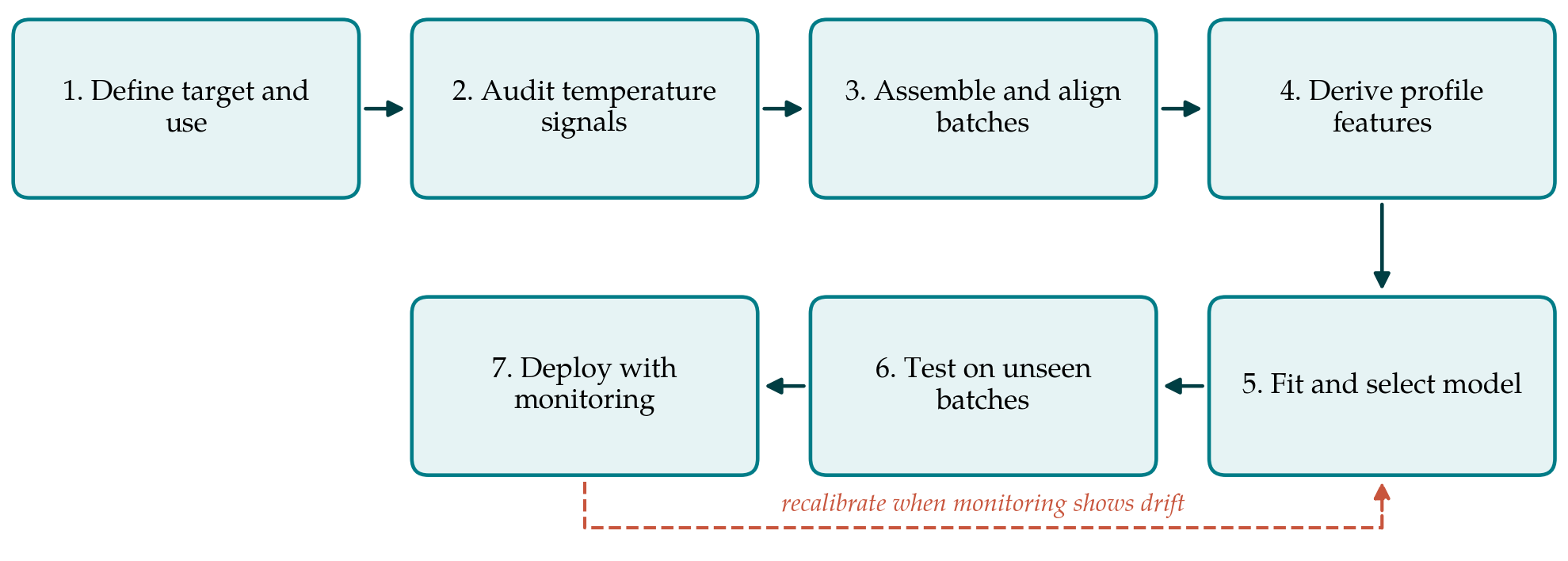
4.1. Step 1: Define the inference target and its use
The designer first states which composition variable is to be inferred, at what points in the batch, and what decision the estimate will support: detecting the end point, timing a feed, or releasing the batch to the next operation. The required accuracy follows from the decision. It should be compared at once with the repeatability of the laboratory method that will supply reference values, since no model can be shown to be more accurate than its reference.
4.2. Step 2: Audit the temperature signals
Each temperature sensor is checked for location, calibration, resolution and response time, and the historian is checked for compression settings that may have flattened the recorded signals. The jacket temperature difference is often a small number obtained from two large ones, so matched and recently calibrated sensors matter more there than anywhere else. Jacket flow should be measured or shown to be constant. Signals that cannot be trusted are excluded at this stage and not left for the regression to sort out.
4.3. Step 3: Assemble and align historical batches
Batches of the same product and recipe are collected together with their laboratory results and the times at which samples were taken. Batches differ in duration, so their trajectories must be brought onto a common basis before they can be compared. Two approaches are established: replacing time with an indicator variable that advances monotonically through the batch, such as the cumulative amount fed, and dynamic time warping, which stretches and compresses trajectories to match a reference (Kassidas et al., 1998). Abnormal batches are identified and set aside or labelled. The calibration set should span the variation the sensor will meet in raw materials, charge sizes and seasons.
4.4. Step 4: Derive features from the profiles
Feeding raw trajectories to a regression is possible, as multiway PLS shows, but with few reference values it invites overfitting. The proposal is to compute a small number of features that the energy balance says should matter. The main one is the cumulative heat released up to the sampling time, obtained from the accumulation term and the jacket duty and normalised by the charge. Others are the current rate of heat release, the temperature difference between reactor and jacket, the elapsed value of the indicator variable, and the heat removed during any feed period. An apparent heat transfer coefficient estimated during a non-reactive phase of the batch, such as initial heating, can be included to let the model compensate for fouling and fill level.
4.5. Step 5: Fit and select the model
A PLS regression is fitted from the features to the laboratory composition. The number of latent variables is chosen by cross-validation, and the unit left out in each round must be a whole batch. Samples from one batch are strongly correlated, and leaving out single samples gives an estimate of error that is far too optimistic, a point made in general terms in the statistical learning literature (Hastie et al., 2009). A linear model should be tried first. If residuals show structure against conversion, a transformation of the output or a model fitted separately to each phase of the batch is preferable to an unconstrained nonlinear learner, given how few reference points are usually available.
4.6. Step 6: Test on unseen batches
A set of batches, ideally the most recent, is withheld from every earlier step, including feature choice. The model is applied to them once. The error is reported against the target set in step 1 and beside the laboratory repeatability, with residuals plotted against time in batch and against calendar date. A model that meets the target on average but fails late in the batch, where end-point decisions are made, has not passed.
4.7. Step 7: Deploy with monitoring and maintenance
On line, the sensor should report not only an estimate but an indication of whether the current inputs resemble those it was built on. The usual tools are the Hotelling statistic and the residual statistic of the latent variable model, as used in multivariate process monitoring (Wise and Gallagher, 1996). When either exceeds its limit the estimate is flagged as unreliable. Routine laboratory samples continue at a reduced frequency and are compared with the estimate. A stated rule, for example a run of residuals of one sign, triggers recalibration, which returns the designer to step 3 with the enlarged data set.
5. Fitting the Procedure to a Plant
The effort required is modest by design. The calculations need a historian export, the laboratory records and standard chemometric software. What takes time is step 3, because sample times are often recorded by hand and must be reconciled with the trajectory before any regression is meaningful. A plant with many products should begin with the one that has the most batches and the cleanest thermal signal, typically a strongly exothermic reaction with a single dominant pathway. Where a kinetic model already exists, an extended Kalman filter built on it can be run alongside the regression as an independent estimate; disagreement between the two is itself informative.
The estimate should enter operation gradually. A period in which it is displayed but not acted on lets operators and chemists compare it with their own judgement and with laboratory results, and exposes operating situations, such as a late charge or a jacket utility upset, that the calibration set did not contain.
6. Limitations and What Remains to Be Shown
The procedure rests on an assumption that will not always hold: that the thermal signal is dominated by the reaction of interest. For weakly exothermic reactions, for reactors with poor jacket instrumentation, and for product attributes that depend on side reactions, temperature profiles may carry too little information, and no amount of modelling will supply it. Step 1 and step 6 are intended to reveal this early, but the designer should be prepared for the answer that a composition analyser is needed after all.
Because the procedure has not been applied here, its performance is unknown. A validation study would need to show, on at least one industrial reactor, the error achieved on unseen batches relative to laboratory repeatability, the stability of that error over months of operation, and whether the physically derived features of step 4 outperform raw trajectories and a model-based observer on the same data. It would also need to record how often the monitoring of step 7 flagged the estimate and whether the flags were justified.
7. Conclusion
Temperature trajectories are the most available measurements on a batch reactor, and the energy balance explains why they can stand in for composition when one reaction governs the heat release. The design procedure proposed here combines that physical argument with latent variable regression, insists on batch-wise validation, and treats monitoring and recalibration as part of the sensor. Whether it delivers estimates good enough to replace routine sampling is a question for plant trials, which this article is intended to prepare and not to pre-empt.
Conflict of interest
To be declared by the author(s) before publication.
Funding
To be declared by the author(s) before publication.