1. Introduction
The diffusion coefficient of a protein in a living cell looks like a simple physical constant. In practice it is the output of an experiment and a model, and different experiments return different values. In their assessment of nuclear protein dynamics, Mueller et al. (2010) noted that published estimates for the same molecule varied widely between studies and asked how much was really known. The problem is sharpest when the two values come from the same laboratory: a recovery curve from a confocal microscope implies one coefficient, tracks from a camera-based single-molecule instrument imply another, and the two differ by a factor that no error bar covers.
Such a discrepancy can mean three things. One or both measurements may be biased by the instrument or the analysis. The two experiments may not have been performed on the same biological system, despite appearances. Or the protein may move in a way that a single coefficient cannot describe, so that both values are correct for the scale at which they were obtained. Telling these apart requires a sequence of checks carried out in a sensible order, cheapest and most decisive first.
This article sets out such a sequence. It takes as its running illustration the pairing of fluorescence recovery after photobleaching (FRAP) with single-particle tracking (SPT), with fluorescence correlation spectroscopy (FCS) as the arbiter, since these are the three techniques most laboratories have access to. The procedure is a proposal built from published methods. No application to experimental data is reported.
2. What Each Platform Measures
The starting point is that the techniques do not observe the same quantity. Table 1 summarises what each records, the scale it probes and the biases to which it is prone.
| Technique | What is observed | Scale probed | Characteristic biases |
|---|---|---|---|
| FRAP | Refilling of a bleached region by unbleached molecules | Micrometres; seconds | Diffusion during bleaching; binding; finite reservoir (Braeckmans et al., 2003) |
| FCS | Intensity fluctuations in a fixed focal volume | Sub-micrometre; milliseconds | Volume calibration; photobleaching; immobile molecules unseen (Petrášek and Schwille, 2008) |
| SPT, displacement analysis | Mean squared displacement of individual tracks | Tens of nanometres; milliseconds | Localisation error; motion blur; short tracks (Michalet, 2010) |
| SPT, jump-length analysis | Distribution of steps pooled over many short tracks | Tens of nanometres; milliseconds | Fast molecules leave the focal plane (Hansen et al., 2018) |
| All three | Mobility of a labelled protein in a living cell | As above | Temperature; expression level; label; anomalous transport (Weiss et al., 2004) |
In FRAP, fluorescence in a small region is bleached and the return of signal is followed as unbleached molecules move in. The classical analysis of Axelrod et al. (1976) treated a Gaussian beam, and Soumpasis (1983) gave the solution for a uniform circular spot, from which the familiar relation D = 0.224 r2/t1/2 between the coefficient, the spot radius and the half-time of recovery is taken. Both assume an instantaneous bleach, an effectively infinite two-dimensional pool and pure diffusion. On a laser-scanning confocal microscope the bleach takes time, molecules move while it is applied, and the bleached profile is wider and shallower than the nominal region. Using the nominal radius then underestimates the coefficient (Braeckmans et al., 2003; Kang et al., 2012). When the protein binds to immobile structures, recovery is slowed further, and in the limit of fast exchange the curve still has the shape of diffusion but with an effective coefficient reduced by the bound fraction (Sprague et al., 2004).
Tracking follows individual molecules, and the coefficient is usually obtained from the slope of the mean squared displacement against time (Qian et al., 1991). The intercept of that line contains the localisation error, and movement during the camera exposure subtracts a further term, so slopes fitted to the first few points can be biased in either direction unless both effects are modelled (Berglund, 2010; Michalet, 2010). Tracking also selects. Fast molecules blur, are harder to localise and leave the focal plane within a frame or two, so the population of long tracks is enriched in slow and bound molecules (Hansen et al., 2018). FRAP reports a population average over micrometres and seconds, while tracking reports on tens of nanometres and milliseconds for the molecules it manages to follow. Agreement between them is not to be expected without care.
3. The Proposed Procedure
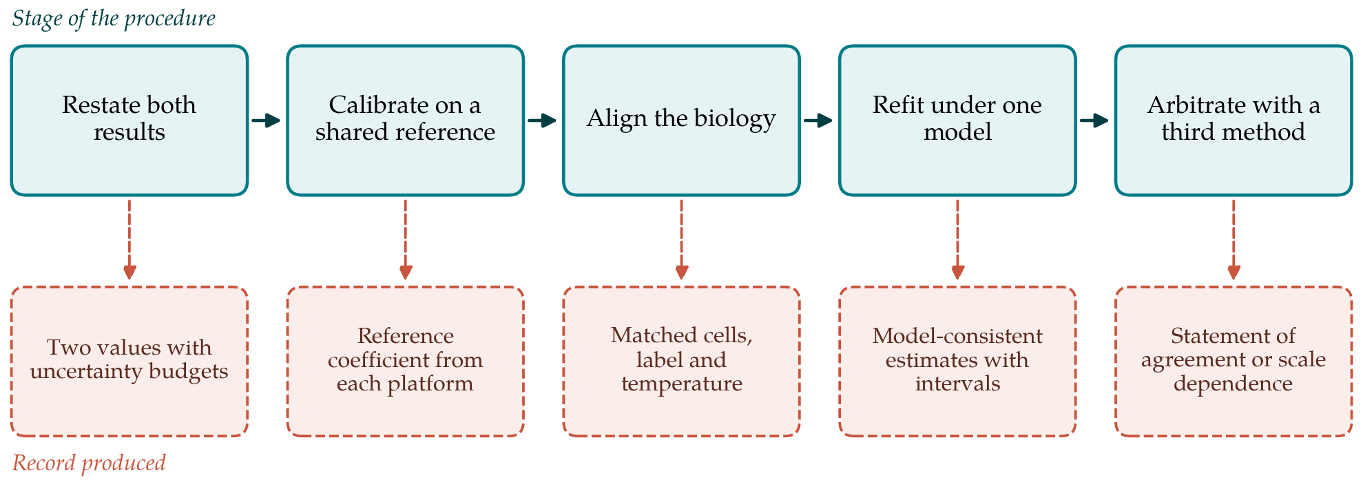
The procedure has five stages, shown in Figure 1 with the record that each should leave. The order is deliberate. Early stages cost little and can dissolve the discrepancy entirely, while later stages need new experiments and are worth doing only once the simpler explanations have been excluded.
3.1. Restating the two results with their uncertainties
Many apparent conflicts are between numbers whose uncertainty was never worked out. The first stage is to write each result as a value with an uncertainty budget in the manner of the Guide to the Expression of Uncertainty in Measurement (JCGM, 2008): a list of inputs, the uncertainty of each and its contribution to the result. For FRAP the inputs include the effective bleach radius, which enters as a square, the frame time and the fitting model. For tracking they include the pixel size, the frame interval, the localisation precision and the number and length of tracks. Variation between cells is reported separately from variation within a cell, with the cell as the unit of replication. If the two intervals overlap once this is done, the matter ends here.
3.2. Calibrating each platform against a shared reference
The second stage asks whether each instrument returns the right answer for a sample whose answer is known. A solution of a fluorescent dye, or of purified fluorescent protein in a glycerol-water mixture of known viscosity that slows it into the measurable range, is measured on both platforms at the same recorded temperature. Care is needed over the reference value itself: scanning FCS measurements that do not rely on knowledge of the focal volume showed that coefficients long quoted for common calibration dyes were too low (Petrášek and Schwille, 2008). Temperature must be controlled closely, because the Stokes-Einstein relation makes the coefficient proportional to absolute temperature divided by viscosity, and the viscosity of water falls steeply enough that a small solute diffuses roughly a third faster at 37 °C than at 25 °C. A platform that fails on the reference sample has a calibration problem that must be solved before any cellular data are compared.
3.3. Aligning the biological conditions
The two experiments are then examined for differences in what was measured. Tracking generally needs sparse labelling and often a different tag, such as a self-labelling enzyme domain with an organic dye, from the fluorescent protein fusion used for FRAP. The tag changes size and may change behaviour. Expression level matters where binding sites can be saturated, since the bound fraction then depends on concentration. Stage temperature, medium, time after plating, cell-cycle stage and the subcellular region chosen all alter mobility. The third stage draws up a side-by-side list of these conditions and repeats whichever experiment is easier with the conditions matched. An inert tracer measured on both platforms in the same cells, for which unfused fluorescent protein is the conventional choice (Swaminathan et al., 1997), separates effects of the cellular environment from effects specific to the protein of interest.
3.4. Refitting both data sets under a shared model
If a gap remains, the fourth stage replaces the two default analyses with one physical model applied to both data sets. For a protein that binds, the model has at least a free coefficient, an association rate and a dissociation rate. The FRAP curve is fitted with a reaction-diffusion solution and the measured post-bleach profile in place of the nominal spot (Sprague et al., 2004; Kang et al., 2012). The tracking data are fitted with a two-state displacement model that includes localisation error, motion blur and loss of fast molecules from focus (Hansen et al., 2018). The comparison is then between like quantities: free coefficient with free coefficient, bound fraction with bound fraction. A single coefficient from a FRAP half-time and a single slope from pooled tracks are not like quantities when the protein spends part of its time bound.
3.5. Arbitrating with a third measurement
The last stage brings in a technique with different weaknesses. FCS observes fluctuations in a diffraction-limited volume at nanomolar concentrations and is blind to immobile molecules, which makes it a useful check on the free coefficient. Two published exercises show what such arbitration looks like. Stasevich et al. (2010) used FRAP and FCS to test each other on the same proteins and traced their initial disagreement to photobleaching. Mazza et al. (2012) compared FRAP, FCS and single-molecule tracking for one transcription factor and showed how conflicting binding estimates could be brought into line. Agreement between any two methods should be judged as Bland and Altman (1986) recommended for clinical measurements, by examining differences against means across cells, and not by a correlation coefficient, which can be high when two methods disagree systematically.
4. Interpreting a Difference That Survives
A discrepancy that persists after calibration, matching, joint modelling and arbitration deserves to be taken seriously as a property of the system. The interior of a cell is crowded and structured, and tracer motion in it is frequently subdiffusive: the mean squared displacement grows more slowly than linearly with time (Weiss et al., 2004; Höfling and Franosch, 2013). Under those conditions an apparent coefficient depends on the distance and time over which it is measured, and a method that probes micrometres will return a lower value than one that probes tens of nanometres. Transient confinement, hopping between compartments and binding with a broad range of residence times have the same effect. The appropriate report is then not a reconciled number but both values, each with its length and time scale, together with the exponent or model that connects them.
5. Limitations and What Remains to Be Shown
The procedure is a proposal. It has not been validated in this article, and its usefulness depends on claims that should be tested: that the ordering of stages does resolve most discrepancies early, that the shared-model stage is identifiable with data of ordinary quality, and that the effort is proportionate. Joint models with several rate constants can fit well and still be poorly constrained, and a good fit on both platforms does not prove the model. A reference sample validates an instrument under ideal optical conditions, and aberrations deep in a cell may differ. The illustration used here involves FRAP and tracking; other pairings, such as two tracking systems with different cameras or image correlation methods against point FCS, would need their own lists of biases. A natural test would be a planned comparison in which one construct is measured on several platforms by the staged procedure and by default analyses, with the spread of estimates compared between the two.
6. Conclusion
Two diffusion coefficients for one protein are a prompt for investigation and not an embarrassment to be managed by choosing between them. The staged procedure proposed here moves from bookkeeping to calibration to biology to modelling to independent arbitration, and leaves a written record at each point. Its premise is that most disagreements have mundane causes that can be found, and that those that cannot be explained away are informative about how the molecule moves. Whether the procedure delivers that in practice is for laboratories with access to several platforms to establish.
Conflict of interest
To be declared by the author(s) before publication.
Funding
To be declared by the author(s) before publication.