1. Introduction
Safety stock is the inventory held beyond expected requirements to cover the chance that demand during the replenishment lead time exceeds its mean. In a continuous review system the reorder point is the expected lead time demand plus a multiple of its standard deviation, and the multiple is read from the normal distribution for the service level wanted. When lead time is itself uncertain, the variance of lead time demand is taken as the sum of two terms: the mean lead time multiplied by the variance of per-period demand, and the square of mean per-period demand multiplied by the variance of lead time. The expression goes back to the classical treatment of Hadley and Whitin (1963) and appears in every operations text (Silver et al., 2017).
The derivation needs three things to be true. Demands in different periods must be independent and identically distributed. The lead time must be independent of those demands. And the resulting total must be close enough to normal for a normal quantile to be meaningful. Planners who use the formula seldom test any of these, and enterprise planning systems apply it to thousands of items without comment.
This article sets out a procedure for the items where the assumptions are doubtful and the cost of error is large. It estimates the distribution of lead time demand, or the service achieved by a given reorder point, by simulation from the firm's own records, preserving whatever dependence those records contain. The procedure is proposed here for discussion and trial. No application to operational data is reported.
2. Background
The procedure draws on what is known about the failure of the standard formula, on the forms that dependence takes in replenishment data, and on methods for generating dependent inputs in simulation.
2.1. Where the standard formula fails
Doubts about the normal approximation are old. Eppen and Martin (1988) showed with simple examples that when lead time takes a few discrete values, as it does when shipments arrive on particular sailings, the distribution of lead time demand is multimodal and the formula can give reorder points that are badly wrong. Bagchi et al. (1986) examined how lead time variability changes the shape of that distribution. Chopra et al. (2004) demonstrated that for moderate service levels the normal approximation gets even the direction of the effect wrong: reducing lead time uncertainty can increase the safety stock truly required, although the formula says the opposite. Tyworth and O'Neill (1997) offer the counterweight, finding the approximation reasonably robust in cost terms for the distribution settings they studied. The fair summary is that the formula is adequate for many items and unreliable for an identifiable minority.
2.2. Forms of dependence
Table 1 lists the kinds of dependence that matter. Two deserve emphasis. Demand that is positively autocorrelated, as under promotions or trends, accumulates over a lead time with more variance than independent demand of the same per-period spread, so the first term of the formula is too small. And demand may be correlated with lead time. A supplier serving many customers in the same market is busiest exactly when each of them is ordering most, and its lead times lengthen with the load. Wang et al. (2010) treat this case and show that ignoring the correlation mis-sizes the inventory, with too little stock when the correlation is positive. General treatments of stochastic lead times are given by Zipkin (2000) and Axsäter (2015).
| Form of dependence | Typical cause | Effect if ignored | Treatment |
|---|---|---|---|
| Autocorrelated demand | Promotions, trends, customer ordering habits | Variance over the lead time understated | Resample demand in blocks or fit a time series model |
| Demand and lead time correlated | Supplier congestion when the market is busy | Stock too low if positive, too high if negative | Paired resampling or a copula |
| Seasonal co-movement | Peak season affects orders and transport together | Annual average hides peak-season risk | Stratify records by season |
| Lumpy lead times | Fixed sailings, batch production, customs holds | Multimodal lead time demand | Use the empirical lead time distribution |
| Order crossover | Later orders arrive before earlier ones | Effective lead time misjudged | Simulate individual orders and receipts |
2.3. Generating dependent inputs
Simulation input modelling offers two families of method. The first resamples the data. The bootstrap of Efron and Tibshirani (1993) was applied to reorder levels by Bookbinder and Lordahl (1989), and Willemain et al. (2004) used a bootstrap that respects autocorrelation to forecast lead time demand for intermittent service parts. The second family fits marginal distributions to each variable and joins them with a dependence structure. A copula does this in general form (Nelsen, 2006), and the rank-based method of Iman and Conover (1982) imposes a target rank correlation on samples drawn from arbitrary marginals. Biller and Nelson (2003) extend the idea to inputs that are correlated both across variables and over time. A related empirical line sets safety stock from the observed distribution of forecast errors instead of a theoretical one (Trapero et al., 2019).
3. The Proposed Procedure
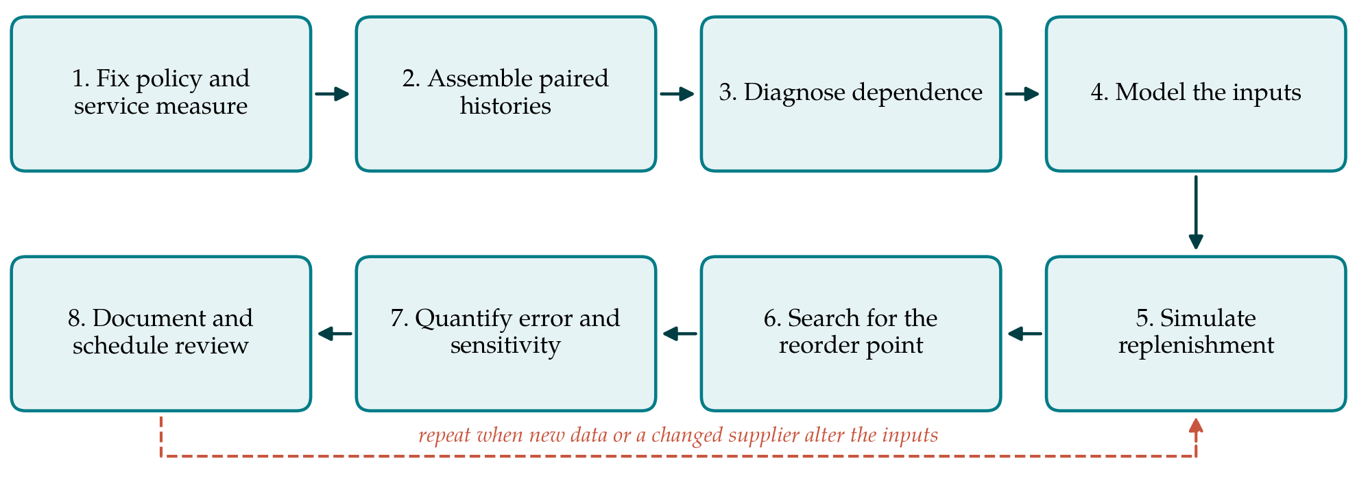
The eight steps are shown in Figure 1 and described below. The procedure is meant for selected items, typically those with high value, long or erratic lead times and a history of either stock-outs or persistent excess. For the remainder the formula can stay.
3.1. Step 1: Fix the policy and the service measure
The simulation must imitate the rule actually used: continuous review with a reorder point and fixed order quantity, or periodic review with an order-up-to level. The service measure must be stated with equal care, because cycle service level, the probability of no stock-out in a replenishment cycle, and fill rate, the fraction of demand met from stock, lead to different stock levels for the same nominal percentage (Silver et al., 2017).
3.2. Step 2: Assemble paired histories
For each item the analyst extracts per-period demand and, for every replenishment order, the date placed and the date received. The essential point is pairing: each observed lead time is kept with the demand that occurred while it ran. Demand should be true demand where it is recorded, since sales censored by stock-outs understate the upper tail. Lead time is measured to availability for use, including inspection and put-away. Periods affected by one-off events are flagged and a decision on their inclusion is recorded.
3.3. Step 3: Diagnose dependence
Before any model is chosen the data are examined. The autocorrelation function of demand shows whether periods can be treated as independent. A scatter plot and a rank correlation coefficient between each lead time and the average demand rate during it show whether the two move together. Splitting the records by season or by supplier shows whether an apparent correlation is merely a mixture of regimes. If none of these checks reveals structure and the lead time distribution is unimodal, the formula is probably adequate and the procedure can stop.
3.4. Step 4: Model the inputs
Where the history is long enough, the simplest defensible model is to resample it. Whole replenishment cycles, each consisting of a lead time and the run of demands observed during it, are drawn with replacement, which carries both the autocorrelation within the cycle and the link between demand and lead time into the simulation without any distributional assumption. Its weakness is that it cannot produce a value more extreme than the worst on record. Where history is short, marginal distributions are fitted to demand and to lead time and joined by a copula with the rank correlation estimated in the previous step. The choice of copula family affects the joint upper tail, which is the region that determines safety stock, so it should be varied in the sensitivity analysis and not treated as settled.
3.5. Step 5: Simulate the replenishment process
With the input model in place, the inventory policy is run period by period for a long horizon: demand is drawn, stock is decremented, an order is released when the inventory position reaches the reorder point, and its lead time is generated consistently with the demand regime in force. Outstanding orders are tracked individually so that crossover is represented. For the special case of cycle service under continuous review it is enough to simulate lead time demand directly. Standard practice applies: a warm-up period is discarded, several independent replications are run, and the same random number streams are used for every candidate reorder point so that differences between candidates are not noise (Law, 2015).
3.6. Step 6: Search for the reorder point
For cycle service the answer is a quantile: the reorder point is the value that simulated lead time demand exceeds in the permitted fraction of cycles. For fill rate there is no such shortcut, and the reorder point is found by search. Because service does not decrease as the reorder point rises, bisection over a bracketing interval converges quickly when common random numbers are used. Safety stock is the reorder point less the mean of simulated lead time demand. More elaborate simulation optimisation methods exist (Fu, 2002) and are unnecessary for a single parameter.
3.7. Step 7: Quantify error and sensitivity
A simulated reorder point carries two kinds of uncertainty. Monte Carlo error, from the finite number of runs, is measured by the spread across replications and reduced by running more. Input uncertainty, from the finite history, is usually larger and is ignored more often. It can be gauged by bootstrapping the history itself: resample the records, refit the input model, repeat the search, and observe how far the reorder point moves (Efron and Tibshirani, 1993). The analyst should also rerun the search with the dependence removed, which shows how much of the stock is attributable to correlation, and with alternative copula families or block lengths.
3.8. Step 8: Document and schedule review
The result is recorded with the data window, the exclusions, the input model, the number of replications, the interval from the previous step and the comparison with the formula value. A review date is set, and a review is also triggered by a change of supplier, route or order quantity, any of which alters the lead time process on which the calculation rests.
4. Fitting the Procedure to Practice
The computation is light and can be done in a spreadsheet with a scripting language or in any statistical package. The practical obstacles lie elsewhere. Receipt dates are often recorded less carefully than order dates, and many systems overwrite the planned lead time instead of storing each actual one. An item ordered six times a year yields few lead time observations, and pooling across similar items from the same supplier and lane is then the only way to obtain a usable sample. Finally, the parameter the planning system accepts is usually a safety stock quantity or a number of days of cover, so the simulated reorder point has to be translated into that form and protected from being overwritten by the system's own calculation.
5. Limitations and What Remains to Be Shown
The procedure has not been tested, and three questions are open. The first is whether it outperforms the formula out of sample: reorder points set from one period of history should be judged on the service they deliver in the next, and a method that fits the past closely may do no better than a crude one when the future differs. The second is how much history is needed before the estimate of dependence is stable enough to act on, since a rank correlation computed from a dozen cycles has a wide interval. The third is cost. The effort is justified only for items where the difference in stock is material, and a rule for selecting those items in advance is itself something to be developed.
There are structural limits as well. The procedure treats one item at one location and takes the order quantity as given. It does not address stock held at several echelons, items that share a container or a supplier's capacity, or demand that responds to availability. It also inherits the stationarity assumption of all history-based methods: if the dependence between demand and lead time arises from a supplier's congestion, a change of supplier removes it.
6. Conclusion
Where demand and lead time are correlated, autocorrelated or lumpy, the usual safety stock formula rests on assumptions the data contradict. Simulation from paired records offers a direct alternative that keeps the dependence present in the firm's own history and reports the uncertainty of its answer. The eight steps proposed here are deliberately plain, and they begin with a diagnosis that sends most items back to the formula. Their merit relative to simpler practice awaits out-of-sample testing on operational data.
Conflict of interest
To be declared by the author(s) before publication.
Funding
To be declared by the author(s) before publication.