1. Introduction
A reported concentration of lead in a water sample or of cadmium in a soil digest is an estimate, and the user of the result needs to know how far the true value might lie from it. The Guide to the Expression of Uncertainty in Measurement gave that idea a formal shape: every result should be accompanied by a quantitative statement of its uncertainty, built from standard uncertainties that are combined by the law of propagation (JCGM, 2008). The international standard for testing laboratories makes the evaluation a condition of accreditation (ISO, 2017a), and regulators increasingly ask for the uncertainty when a result is compared with a limit.
Inductively coupled plasma optical emission spectrometry (ICP-OES) is the routine technique for metals in waters, soils, foods and industrial materials. A typical laboratory reports twenty or more elements per sample, in several matrices, across concentrations that span orders of magnitude. Building a separate uncertainty budget for each combination from first principles is beyond the time most laboratories can give, and the budgets that do get written are often dominated by the tolerances of balances and volumetric flasks, which are easy to quantify and small, while digestion recovery and matrix effects, which are difficult to quantify and large, are left out.
This article sets out a procedure by which a routine laboratory can estimate uncertainty for ICP-OES results from data it already collects. The procedure is assembled from published guidance and is proposed for adoption. It has not been validated here against an independent estimate, and its limits are discussed.
2. Background
Two matters need to be understood before the steps are described: the choice between the modelling and the empirical routes to an uncertainty estimate, and the features of plasma emission measurement that generate uncertainty.
2.1. Two routes to an estimate
The modelling route writes the result as a function of input quantities, assigns a standard uncertainty to each and propagates them. It is the approach of the original guide and is worked through for chemical examples in the Eurachem/CITAC guide (Ellison and Williams, 2012). The empirical route starts from the observed performance of the whole method. It combines a precision term obtained under conditions that vary everything likely to vary in routine use with a term for bias, and it was developed in detail by Ellison and Barwick (1998) and in the Nordtest handbook (Magnusson et al., 2017). ISO has since published standards on the use of validation and quality control data for the purpose (ISO, 2012; ISO, 2017b), and the Eurolab report on alternative approaches treats the routes as equally legitimate when properly applied (Eurolab, 2007).
For a multi-element routine method the empirical route has a practical advantage. Its inputs are produced every working day, so the estimate rests on many observations and can be kept current. Its weakness is that it describes the samples used to generate the data, and those samples may not represent every sample the laboratory receives.
2.2. Where uncertainty arises in ICP-OES
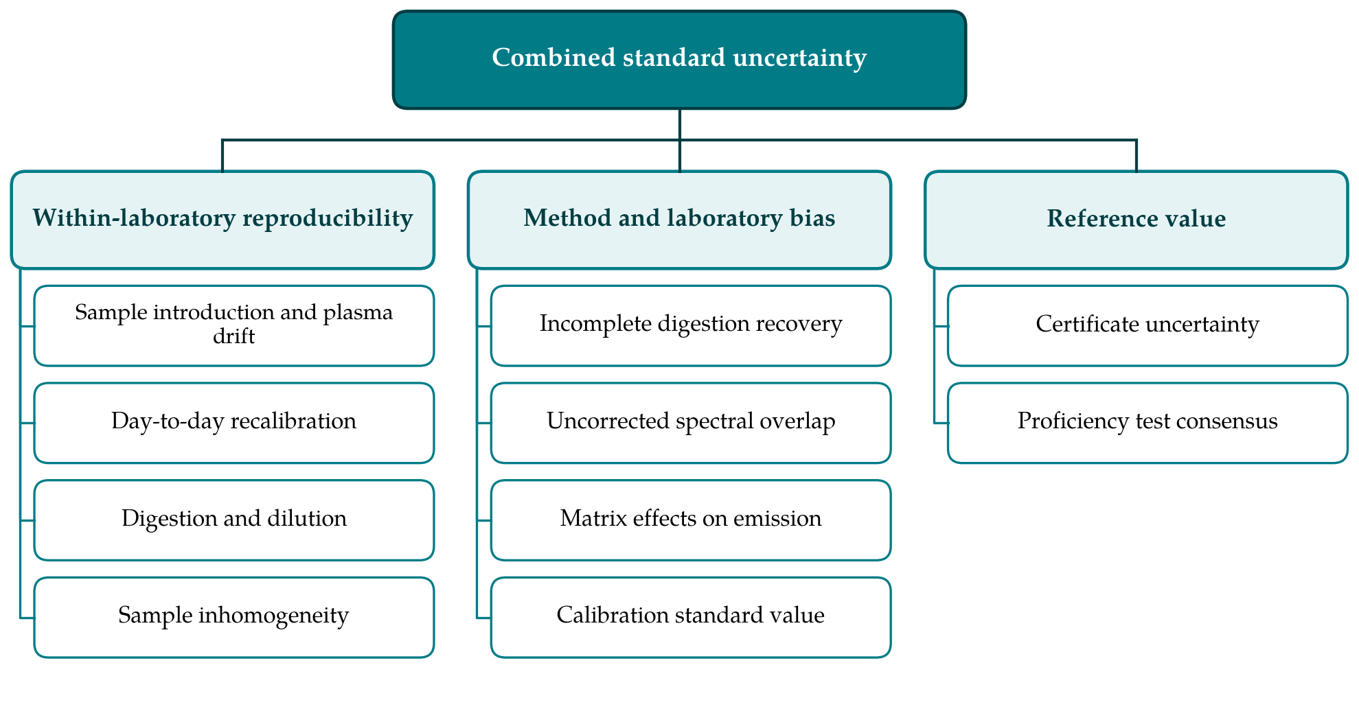
An ICP-OES result passes through sampling of the laboratory portion, digestion or dilution, nebulisation, excitation in the plasma, measurement of line intensity above background, and calibration. Each stage contributes. Nebuliser and torch behaviour drift over a run and change with dissolved solids. High concentrations of sodium, calcium and other easily ionised elements alter excitation conditions and shift analyte signals, an effect that depends on plasma robustness and viewing mode (Todolí et al., 2002). Mermet (1991) proposed the ratio of a magnesium ionic line to a magnesium atomic line as a simple indicator of that robustness. Spectral overlap from matrix elements such as iron and aluminium biases results at weak analyte lines unless corrected. Standard methods for the technique describe these interferences and the controls expected, including internal standards and interference check solutions (US EPA, 1994; ISO, 2007). Figure 1 groups the sources under the terms used in the procedure below.
3. The Proposed Procedure
The procedure has seven steps. Steps 1 and 2 define the problem, Steps 3 to 5 produce the estimate, and Steps 6 and 7 test and maintain it.
3.1. Step 1: Specify the measurand and the ranges
The laboratory states what is being measured: the element, the matrix group, and whether the result refers to total content or to the fraction released by a defined digestion, such as an aqua regia extract. The distinction decides what counts as bias later. The working range of each element is then divided where necessary, because uncertainty near the limit of quantification is roughly constant in concentration units while at higher levels it is roughly proportional to concentration. The Eurachem guide describes how the two regimes may be represented (Ellison and Williams, 2012). In practice a low range expressed in absolute terms and a high range expressed in relative terms is usually enough.
3.2. Step 2: Map the sources and check coverage
A cause-and-effect diagram of the kind shown in Figure 1 is drawn for the method, and each source is marked according to whether the laboratory's quality control data would capture it. A control sample introduced only at the instrument does not capture digestion. A synthetic control solution does not capture matrix effects. A control analysed once per batch does capture recalibration and day-to-day drift. The purpose of the map is to prevent both omission and double counting, and it is the one place where the reasoning of the modelling route is retained.
3.3. Step 3: Estimate within-laboratory reproducibility
The precision term is the standard deviation of results for a stable control sample analysed over a long period, by different analysts, with fresh calibrations, and carried through digestion where the method includes it. Several months of data from the control chart are normally available. If the control sample is simpler than routine samples, a second contribution is added from duplicate analyses of real samples, which reflect inhomogeneity and matrix-dependent variation (Magnusson et al., 2017). Separate values are obtained for the low and high ranges defined in Step 1. Outlying control results that were investigated and attributed to an identified fault may be excluded; results that were merely inconvenient may not.
3.4. Step 4: Estimate the uncertainty arising from bias
Bias is assessed against the best reference values available, and Table 1 compares the three usual sources. Certified reference materials of matching matrix give the most direct evidence. Proficiency test results extend the evidence to more matrices and levels, at the cost of a less certain assigned value. Recovery of a spike added before digestion covers elements and matrices for which nothing else exists, though an added solution may be recovered more easily than the native analyte (Barwick and Ellison, 1999).
| Source | What it covers | What it does not cover | Uncertainty of the reference value |
|---|---|---|---|
| Matrix certified reference material | Digestion, matrix effects, calibration, for that matrix and level | Other matrices and concentration levels | From the certificate |
| Proficiency test rounds | Whole method on realistic samples at several levels | Matrices outside the scheme | From the scheme report; larger for consensus values |
| Spike recovery before digestion | Losses and matrix effects on added analyte | Release of analyte bound in the solid | From spike preparation |
| Second-source calibration check | Error in calibration standards | Everything before the instrument | From the standard certificate |
| Interference check solution | Uncorrected spectral overlap at chosen lines | Non-spectral matrix effects | Not applicable: a pass or fail control |
The component is calculated in the manner of the Nordtest handbook. Where several reference materials or proficiency rounds are available, the root mean square of the observed relative biases is combined in quadrature with the mean standard uncertainty of the reference values. Where a single reference material is used, the observed bias, the standard deviation of its mean and the certificate uncertainty are combined in the same way. The harmonised validation guidelines advise that a bias found to be significant should be investigated and removed if possible (Thompson et al., 2002); a bias that is understood and stable may be corrected, and its contribution then falls to the uncertainty of the correction.
3.5. Step 5: Combine and expand
The combined standard uncertainty is the square root of the sum of the squared reproducibility and bias
2 + ubias
2)1/2. It is multiplied by a coverage factor of 2 to give an expanded components, uc = (uRw uncertainty with a level of confidence of approximately 95 per cent, on the assumption that the components rest on enough observations for a normal distribution to be reasonable (JCGM, 2008). The calculation is made for each element, matrix group and range. Elements that behave alike may be grouped under the largest value in the group to keep the reporting table manageable, provided the grouping is recorded.
3.6. Step 6: Check plausibility
An estimate should be tested before it is used. Three checks are proposed. The first compares the relative uncertainty with what interlaboratory experience predicts at that concentration. The Horwitz function (Horwitz, 1982), with the modification proposed by Thompson (2000) for low concentrations, gives a reproducibility standard deviation that a single laboratory should not normally exceed and is unlikely to better by a wide margin. The second examines the laboratory's own proficiency test record: if the claimed uncertainty were correct, the differences from the assigned values should mostly lie within it. The third applies the modelling route to one or two elements as a cross-check, for which the spreadsheet method of Kragten (1994) is convenient. Marked disagreement in any check sends the analyst back to Step 2.
3.7. Step 7: Report and review
The expanded uncertainty is reported with the result, in the same units, with the coverage factor stated. The laboratory records which data sets were used and over what period. The estimate is recalculated at a fixed interval, annually in most cases, and whenever the method changes in a way that Step 2 shows to be relevant: a new digestion procedure, a change of viewing mode, a different internal standard or a new sample type.
4. Fitting the Procedure to a Routine Laboratory
The procedure asks for little that an accredited laboratory does not already do, but it does ask that quality control be designed with uncertainty in mind. The control sample should be a real matrix, or as near to one as stability allows, and should enter the method at the first step. Control concentrations should sit in both the low and the high range for the elements that matter most. Proficiency schemes should be chosen to cover the matrices on the scope of accreditation. With those conditions met, the calculation itself fits on a single spreadsheet per method, and its upkeep becomes part of the periodic review of control charts.
Sampling outside the laboratory is not included. Where the customer's question concerns a field, a batch or a water body and not the portion delivered, the uncertainty of sampling may exceed everything discussed here and has to be addressed separately.
5. Limitations and What Remains to Be Shown
The procedure is a proposal and is not validated in this article. Its main assumption is that the control samples, reference materials and proficiency samples behave as routine samples do. For a laboratory with a narrow and stable sample stream the assumption is reasonable. For one that receives unusual matrices, such as brines, high-iron sludges or organic-rich digests, the estimate will be too small for those samples, and individual assessment remains necessary. The bias component is also sensitive to the number and quality of reference values: a handful of proficiency rounds with consensus assigned values gives a weak estimate.
What would need to be demonstrated is whether estimates obtained in this way agree, element by element, with full modelling budgets and with the spread observed in collaborative trials, and how stable they are from one review period to the next. Such comparisons can be made with data that laboratories already hold and would be a useful subject for a follow-up study.
6. Conclusion
For routine multi-element analysis by ICP-OES, an uncertainty estimate based on long-term control data and on evidence of bias is more complete and easier to maintain than a budget assembled from individual tolerances. The seven steps proposed here keep the cause-and-effect analysis as a check on coverage, separate the low and high concentration regimes, and require the estimate to be tested against independent benchmarks before it is reported. The approach makes plain where a laboratory's quality control is too thin to support the uncertainty it claims, which is itself a useful result.
Conflict of interest
To be declared by the author(s) before publication.
Funding
To be declared by the author(s) before publication.