1. Introduction
The whole-farm budget is the basic instrument of farm management. It sets the expected receipts of every enterprise against variable costs to give gross margins, deducts overheads and finance charges, and arrives at a net farm income for the year (Kay et al., 2016). Its weakness is equally basic. Prices and yields are entered as single values, although the farmer knows them only as ranges, and the answer inherits a precision that the inputs never had. In years of volatile commodity and input prices the gap between the budgeted figure and the realised one can decide whether a loan is repaid.
Stochastic budgeting addresses the weakness directly. The uncertain entries are described by probability distributions, values are drawn from them repeatedly, and the budget is recalculated for each draw, giving a distribution of profit in place of a point (Hardaker et al., 2015). Lien (2003) showed how the approach supports whole-farm decisions over several years. The difficulty for most advisers is the data. Textbook treatments estimate distributions from ten or more years of farm records. A typical family farm can offer a few seasons of sale receipts and a clear memory of the best and worst years.
This article proposes a way of carrying out stochastic budgeting under those conditions. It is aimed at advisers, lenders and students who can build a budget in a spreadsheet. No farm data are analysed and no results are reported. What follows is a procedure and the argument for each of its parts.
2. Background
The procedure draws on two strands of earlier work: decision analysis in agriculture, which legitimises the use of judgement where data are short, and simulation methods that keep the computation honest.
2.1. Probabilities from judgement
Agricultural decision analysis has long held that the probabilities relevant to a farm decision are the decision maker's own degrees of belief, informed by whatever data exist, and that sparse data are a reason to combine evidence with judgement and not a reason to abandon probabilistic reasoning (Anderson et al., 1977). Judgement has well-documented faults. People anchor on an initial value, give too much weight to vivid recent events and state ranges that are too narrow (Tversky and Kahneman, 1974). Structured elicitation methods have been developed to reduce these faults, and the guidance on them is detailed (O'Hagan et al., 2006).
2.2. Simulation with few data
Several technical results make simulation workable when data are thin. Richardson et al. (2000) set out a procedure for simulating correlated farm variables from short series using empirical distributions, without assuming normality. Their caution about distributional form is supported by Just and Weninger (1999), who showed that the evidence on the shape of crop yield distributions is sensitive to how trends are removed. Latin hypercube sampling covers the range of each input evenly with far fewer draws than simple random sampling (McKay et al., 1979), and the method of Iman and Conover (1982) imposes a chosen rank correlation on sampled inputs whatever their marginal distributions.
3. The Proposed Procedure
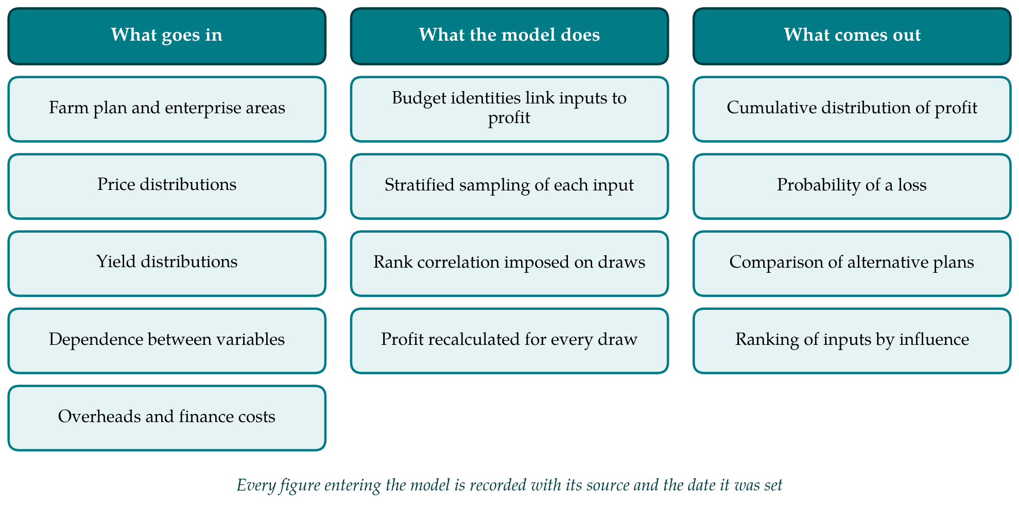
The procedure has six stages. Figure 1 summarises what enters the model, what the model does and what it returns. The stages are described below in the order in which they would be carried out.
3.1. Build the deterministic budget first
The starting point is an ordinary whole-farm budget for the coming year, laid out so that every enterprise gross margin is calculated from an explicit price, yield and area, and so that overheads, interest, lease payments and drawings appear as separate lines. The budget should be checked against the most recent actual accounts, however incomplete. A stochastic model can be no better than the accounting identities beneath it, and errors of structure, such as a forgotten cost or a double-counted by-product, are far more damaging than an imperfect distribution (Pannell, 1997).
3.2. Keep the stochastic variables few
Not every uncertain entry needs a distribution. A one-at-a-time sensitivity test on the deterministic budget, moving each entry between a low and a high value, shows which items move net income appreciably. On most farms these are the prices and yields of two or three main enterprises and the prices of one or two major inputs such as feed, fertiliser or fuel. Restricting the stochastic set to these five to eight variables keeps the elicitation manageable and the correlation structure small enough to specify with care. Everything else stays at its budgeted value.
3.3. Specify each distribution from what is available
Table 1 sets out the options for describing a single variable when records are short. For yields, the farmer's own experience is usually the best source, and a triangular distribution defined by the lowest, most likely and highest values is easy to elicit and to explain. The triangular form is a reasonable stand-in for smoother distributions in applications of this kind (Johnson, 1997). The extremes should be asked for before the most likely value, to limit anchoring, and the farmer should be asked to recall specific bad and good years and what caused them (O'Hagan et al., 2006).
| Approach | Information needed | Strength | Main limitation |
|---|---|---|---|
| Triangular from judgement | Lowest, most likely and highest values | Simple to elicit and explain | Stated ranges are often too narrow |
| Smoothed three-point (beta type) | The same three values | Less weight in the extreme tails | Shape is assumed, not observed |
| Empirical from farm records | Five or more years of own data | Reflects the farm's own conditions | Few points; trends must be removed first |
| Borrowed market series | Published regional or national prices | Long history of variability | Farm price differs by a basis |
| Forecast with historical errors | Outlook or futures price; past deviations | Centred on current information | Past errors may understate new shocks |
| Discrete scenarios | Three to five described states with weights | Easy to discuss with a lender | Coarse; ignores values between states |
Prices are a different matter, because long public series usually exist even when farm records do not. Agricultural prices show trends, seasonal patterns and cycles, and their short-run variation is better measured as deviation from these systematic movements than as raw dispersion (Tomek and Kaiser, 2014). The proposed approach is to take the current outlook price as the centre, to describe variability using percentage deviations of past market prices from their trend, and to adjust for the usual difference between the market quotation and the price the farm receives. Empirical deviations can be sampled directly, as in the approach of Richardson et al. (2000), which avoids choosing a functional form.
3.4. Represent dependence
Treating the variables as independent is the most common error in simple risk models and usually understates risk. Prices of related commodities move together, feed costs follow grain prices, and yields of crops grown in the same season share the weather. Where a farm sells into a local market, yield and price may be negatively related, which dampens revenue variation. With few data, a full correlation matrix cannot be estimated. The procedure asks for a judgement on each important pair, expressed in broad classes such as strongly positive, moderately positive, unrelated or moderately negative, with a numerical rank correlation assigned to each class and checked against any market series available. The resulting matrix is imposed on the samples by the rank-based method of Iman and Conover (1982), after confirming that it is internally consistent (Vose, 2008).
3.5. Sample and compute
Values are drawn by Latin hypercube sampling, and the budget is recalculated for each set of draws. A few thousand iterations are ample for a model of this size, and the adequacy of the number can be tested by repeating the run with a different random seed and confirming that the summary measures barely change. The work can be done in a spreadsheet with a simulation add-in or in a short script. Each run should be stored with its inputs, seed and date so that it can be reproduced when the budget is revisited.
3.6. Read and compare the results
The primary output is the cumulative distribution of net farm income. Three readings are useful to a farmer: the chance that income falls below zero, the chance that it falls below the amount needed to meet debt service and family drawings, and the income exceeded in nine years out of ten. Alternative plans, such as a change in enterprise mix or the forward sale of part of a crop, are compared by plotting their cumulative curves together. Where one curve lies wholly to the right of another the choice is clear (Hadar and Russell, 1969). Where curves cross, the ranking depends on risk attitude, and methods that rank plans over a range of risk aversion can be applied (Meyer, 1977; Hardaker et al., 2004).
4. Checks and Presentation
Three checks are proposed before results are shown to anyone. The first is that the mean of the simulated incomes is close to the deterministic budget; a large difference signals a mistake or a strongly skewed input that needs explaining. The second is that the simulated range is believable to the farmer: if the model says that a loss has a negligible chance and the farmer recalls two losses in the past decade, the ranges are too narrow. The third is a sensitivity analysis on the judgements themselves, widening each elicited range and shifting each correlation class by one step, to see whether the conclusions survive (Pannell, 1997).
A stochastic budget is also a document to be kept. The distributions describe what the farmer and adviser believed at a particular date, and their value grows when they are revisited. At the end of the year the realised prices, yields and income can be marked on the distributions that were set at the start. A single year proves little, since an outcome in the tail of a well-specified distribution will occur now and then. Over several years, however, a farmer whose results fall repeatedly outside the stated ranges has direct evidence that those ranges should be widened, and one whose results cluster near the centre may reasonably narrow them. Keeping this record costs little, and it is the only means by which judgement on an individual farm can be seen to improve.
Presentation should be modest. A cumulative curve with two or three marked thresholds conveys more than a table of moments, and probabilities are better stated as frequencies, such as about one year in five, than to two decimal places. Pannell et al. (2000) argue that in farm modelling the gains from representing risk aversion are often small beside the gains from getting the expected values and the structure of the problem right. The stochastic budget should be offered in that spirit, as a way of seeing the spread around a carefully built central estimate.
5. Limitations and What Remains to Be Shown
The procedure is a proposal and has not been validated here. Its outputs depend on elicited judgements, and no amount of sampling refinement compensates for a range that the farmer has set too tightly. The model covers a single year. It ignores carry-over of stocks and debt, tax, and the adjustments a farmer makes during the season in response to events, all of which a multi-year model would need (Lien, 2003). Borrowed price series may not represent a farm that sells into a thin local market.
A validation would need to show three things. One is calibration: across a set of farms and years, whether realised incomes fall within the central part of the simulated distributions about as often as the distributions say they should. Another is whether elicited distributions differ materially from those estimated on farms that do hold long records. The last is usefulness: whether farmers and lenders shown the distribution make different decisions from those shown the single-figure budget, and whether they regard the difference as an improvement. Each of these can be examined with farm business survey data and cooperating advisers.
6. Conclusion
Short records are a reason to be careful with stochastic budgeting, not a reason to forgo it. By starting from a sound deterministic budget, limiting the stochastic variables to those that matter, combining elicited ranges with public price history, stating dependence explicitly and testing the judgements for their influence on the answer, an adviser can give a farmer a defensible picture of the spread of likely profit. The value of that picture against the single figure it replaces is for empirical work to establish.
Conflict of interest
To be declared by the author(s) before publication.
Funding
To be declared by the author(s) before publication.