International Journal of Signal Processing

Designing Adaptive Beamformers With Few Microphones for Speech Enhancement in Reverberant Rooms: A Methodological Guide

Erik Moreno¹, Tiago Sato², Mateo Nurpeisov³

¹ Department of Electrical Electronics, Volta University Centre for Electrical Electronics, Belgium, ² Department of Electrical Electronics, Irrawaddy Institute of Electrical Electronics, Qatar, ³ Department of Electrical Electronics, Balkan Research Institute of Electrical Electronics, Ethiopia

Published 06 Jul 2026 Vol. 1, Article 3 10.62715/ijsp.2026.v1.i1.pp15-20 0 accesses 0 citations

Download PDF XML HTML EPUB

0Accesses

0Citations

Abstract

Hearing aids, earbuds, laptops and smart speakers carry two to four microphones, and their designers want the directional gain that array processing promises. The classical theory of adaptive beamforming was written for arrays of many sensors in open space. Indoors, with a handful of microphones, two of its assumptions fail: the talker's sound does not arrive as a single plane wave, and there are too few degrees of freedom to null more than one or two interferers. This article proposes a design procedure for that setting. It consists of seven steps: describing the room and the array, fixing the short-time Fourier model, estimating the speech and noise spatial covariance matrices, estimating the relative transfer function of the talker, computing a minimum-variance beamformer with explicit robustness constraints, adding dereverberation and a single-channel postfilter, and evaluating on rooms not used during design. For each step the article gives the reasoning, the choices open to the designer and the published method on which the step rests. The procedure is assembled from the literature as a proposal. It has not been validated experimentally here, and the closing sections state what an evaluation would have to show and where the approach is expected to reach its limits.

Keywords: Adaptive beamforming Microphone arrays Speech enhancement Reverberation Relative transfer function MVDR beamformer

1. Introduction

A beamformer combines the signals of several microphones so that sound from one direction is kept and sound from elsewhere is reduced. Adaptive beamformers choose the combining weights from the data. The minimum-variance design of Capon (1969) minimises output power while passing the wanted direction unchanged, and Frost (1972) showed how to update such a linearly constrained filter sample by sample. The tutorial by Van Veen and Buckley (1988) remains the standard account of this family.

Those methods came from radar, sonar and seismology, where arrays are large and propagation is close to free-field. A consumer device in a living room differs on both counts. With M microphones the beamformer has M - 1 degrees of freedom left after the target constraint, so a two-microphone device can place a single spatial null per frequency. Walls, ceiling and furniture return the talker's voice from every direction over several hundred milliseconds, so that the steering vector computed from geometry no longer describes how the target reaches the microphones. An adaptive beamformer that trusts a wrong steering vector treats part of the speech as interference and cancels it.

The speech enhancement literature has worked out answers to each difficulty, reviewed comprehensively by Gannot et al. (2017). They are scattered across many papers and are seldom presented as a single design path. This article arranges them into a stepwise procedure aimed at arrays of two to four microphones. It reports no experiments. The procedure is proposed, with reasons, for others to apply and test.

2. Background: Why Few Microphones and Reverberation Change the Problem

In a room the sound field of a talker has a direct part, a set of early reflections and a dense late tail. Beyond the critical distance, where direct and reverberant energy are equal, the reverberant part dominates. The late tail is close to a diffuse field, arriving with equal power from all directions, and a small array has little directivity against it, particularly at low frequencies where the microphones are a small fraction of a wavelength apart. The realistic aim for a compact array is therefore to suppress a small number of localised interferers and some of the diffuse noise, and to leave late reverberation of the target to other processing.

Gannot et al. (2001) made the decisive change to the signal model. In place of a steering vector of pure delays, they described the target by the ratios between the acoustic transfer functions to each microphone and that to a reference microphone, the relative transfer function, and they showed that it can be estimated from the microphone signals by exploiting the non-stationarity of speech. With this substitution the constrained beamformer delivers the target as it appears at the reference microphone, reverberation included, and no longer attempts to undo the room. Habets et al. (2010) analysed the resulting trade-off between noise reduction and dereverberation for the minimum-variance beamformer in room acoustics.

3. The Proposed Design Procedure

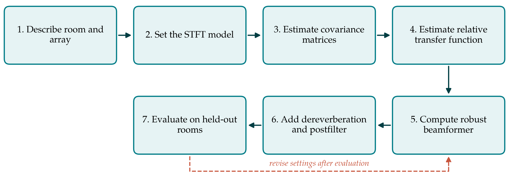
The procedure has seven steps, drawn in Figure 1. Table 1 lists the decision taken at each step and the published method that supports it. The steps are ordered so that each uses only quantities fixed by earlier ones, with a single return path from evaluation to the settings.

Table 1: Steps of the proposed procedure, the decision taken at each and the supporting method
Step	Decision to be taken	Supporting method
1. Room and array	Range of reverberation, distances, noise types; microphone spacing	Image method simulation (Allen and Berkley, 1979)
2. STFT model	Window length, overlap, reference microphone	Multiplicative transfer function model
3. Covariances	How speech absence is detected; averaging constants	Presence probability or mask (Heymann et al., 2016)
4. Relative transfer function	Subtraction or whitening estimator; update rule	Gannot et al., 2001; Warsitz and Haeb-Umbach, 2007
5. Beamformer	MVDR, sidelobe canceller or Wiener form; loading level	Cox et al., 1987; Souden et al., 2010
6. Dereverberation and postfilter	Prediction delay and order; postfilter gain floor	Nakatani et al., 2010; Zelinski, 1988
7. Evaluation	Held-out rooms; objective measures; listening test	Taal et al., 2011; Vincent et al., 2006

Figure 1: The seven steps of the proposed design procedure for a small-array adaptive beamformer

3.1. Step 1: Describe the room and the array

Design starts from the range of conditions the device must handle: the reverberation times of the rooms, the talker distances, the kinds of noise and the number of simultaneous interferers. These fix what can be asked of the beamformer. The array geometry is recorded with its spacings, because spacing above half a wavelength causes spatial aliasing and very small spacing makes the array sensitive to microphone mismatch. For development data, room impulse responses can be generated with the image method of Allen and Berkley (1979) and supplemented by measured responses, with separate sets of rooms reserved for design and for evaluation.

3.2. Step 2: Set the short-time Fourier model

Processing is done per frequency bin of a short-time Fourier transform. The model in which the target at each microphone is the reference signal multiplied by a complex gain holds only if the analysis window is long compared with the significant part of the impulse response. Frame lengths that suit speech are much shorter than typical reverberation times, so the designer has to accept that the multiplicative model captures the direct sound and early reflections and treats the remainder as additional noise. Window length, overlap and the choice of reference microphone are fixed here and kept for all later steps.

3.3. Step 3: Estimate the spatial covariance matrices

Every beamformer in this family is a function of two matrices per frequency bin: the spatial covariance of the noise and that of the noisy mixture or of the speech. They are estimated by recursive averaging of outer products of the microphone vector, with the noise matrix updated when speech is judged absent. The quality of that judgement governs everything downstream. Options run from a voice activity detector, through a speech presence probability computed per time-frequency point, to a mask produced by a neural network trained for the purpose (Heymann et al., 2016). With few microphones the matrices are small and well conditioned after modest averaging, which is one advantage of a compact array.

3.4. Step 4: Estimate the relative transfer function

Two estimators are in common use. Covariance subtraction takes the difference between the noisy and noise covariance matrices as the speech covariance and reads the relative transfer function from its column for the reference microphone. Covariance whitening finds the principal generalised eigenvector of the pair of matrices and maps it back through the noise covariance, an approach that grew out of the blind beamformer of Warsitz and Haeb-Umbach (2007). Whitening is generally the more accurate at low signal-to-noise ratios and costs an eigendecomposition per bin, which for matrices of order two to four is cheap. The estimate should be updated only while the target is active and held otherwise.

3.5. Step 5: Compute the beamformer with robustness constraints

With the relative transfer function in hand, the minimum-variance distortionless response weights follow in closed form from the noise covariance. The same filter can be run in the generalised sidelobe canceller structure of Griffiths and Jim (1982), which separates a fixed beamformer, a blocking matrix that removes the target and an adaptive noise canceller. Souden et al. (2010) give a formulation of the multichannel Wiener filter with a single parameter that moves between the distortionless solution and stronger noise reduction at the cost of some speech distortion, and that does not need the transfer function explicitly.

Robustness has to be designed in, because errors in the transfer function estimate are certain. Diagonal loading of the noise covariance, equivalent to a constraint on white noise gain, limits the amplification of sensor noise and the sensitivity to mismatch (Cox et al., 1987). In the sidelobe canceller form, the blocking matrix can be made adaptive with constrained coefficients so that leaked target is not cancelled (Hoshuyama et al., 1999), and adaptation of the noise canceller is frozen while the target speaks. The loading level is the main tuning parameter of the whole design and is set on the design rooms only.

3.6. Step 6: Add dereverberation and a postfilter

Because the beamformer leaves the target's own reverberation in place, a separate stage is needed if late reverberation is to be reduced. The weighted prediction error method of Nakatani et al. (2010) predicts the late part of each microphone signal from delayed past frames and subtracts it, while a prediction delay protects the direct sound and early reflections. It works with as few as one or two channels and preserves the spatial cues that the beamformer relies on, so it is placed ahead of the covariance estimation. After the beamformer, a single-channel postfilter deals with residual diffuse noise, an arrangement introduced for reverberant rooms by Zelinski (1988). The postfilter gain is given a lower limit to avoid musical noise.

3.7. Step 7: Evaluate on held-out rooms

The design is assessed on rooms, positions and noise recordings that played no part in tuning. Three kinds of objective measure are recommended, since each captures a different failure. Energy-ratio measures separate distortion of the target from residual interference and artefacts (Vincent et al., 2006). Short-time objective intelligibility predicts how much of the speech a listener would understand (Taal et al., 2011), and the perceptual evaluation of speech quality predicts a quality rating (Rix et al., 2001). Each is reported against the unprocessed reference microphone and against a fixed delay-and-sum beamformer. A listening test with human participants should confirm the objective results before any claim about benefit is made.

4. Fitting the Procedure to a Device

Three constraints of real products affect how the steps are carried out. The first is delay. Hearing devices tolerate only a few milliseconds between acoustic and processed sound, which limits the frame length in Step 2 and argues for filter-bank implementations with short windows; a conferencing device can afford much more. The second is computation. Per-bin inversion and eigendecomposition of matrices of order two to four are light, and the dereverberation stage of Step 6 is usually the most expensive component, so it is the first candidate to simplify or omit. The third is the movement of the talker and the device. The forgetting factors of Steps 3 and 4 trade tracking speed against estimation variance, and a head-worn array turns whenever its wearer does.

Where the target direction is known in advance, as with a hearing aid user facing the talker, the estimated transfer function can be combined with a measured or anechoic prior, falling back on the prior when the estimate is unreliable. Where it is not known, a time-delay estimate between microphone pairs, obtained by generalised cross-correlation, can supply an initial steering direction until enough target-dominated frames have been observed.

5. Limitations and What Remains to Be Shown

The procedure is a proposal built from published components, and it has not been applied or validated in this article. Its claims are therefore of design logic and not of measured performance. An evaluation would need to establish, first, that the complete chain improves intelligibility and quality measures over a fixed beamformer across the intended range of reverberation times; second, that target distortion stays low when the transfer function is estimated from short, noisy segments; and third, that the settings chosen on the design rooms carry over to the held-out rooms without retuning.

Some limits are structural and no tuning will remove them. Two microphones cannot cancel two interferers at the same frequency. Diffuse noise at low frequencies is nearly coherent across a compact array and is hard to separate from the target. The whole design depends on deciding when the target is active, and in competing speech that decision is itself the hard problem. Readers applying the procedure should expect the gain to shrink as the talker moves beyond the critical distance and should measure, not assume, how quickly.

6. Conclusion

Adaptive beamforming with a small microphone array in a reverberant room is feasible when the design respects what the array can and cannot do. The procedure proposed here replaces the geometric steering vector with an estimated relative transfer function, builds robustness into the weight computation, assigns late reverberation and diffuse noise to dedicated stages, and insists on evaluation in rooms the designer has not tuned on. Each step rests on an established method, and their combination into one path is what is offered. Whether the combination performs as its logic suggests is a question for experiment, and the evaluation plan in Step 7 is intended to make that experiment straightforward to carry out.

Conflict of interest

To be declared by the author(s) before publication.

Funding

To be declared by the author(s) before publication.

References

[1] Allen, J.B. and Berkley, D.A. Image method for efficiently simulating small-room acoustics. The Journal of the Acoustical Society of America https://doi.org/10.1121/1.382599 65(4), 943-950 (1979).
[2] Capon, J. High-resolution frequency-wavenumber spectrum analysis. Proceedings of the IEEE https://doi.org/10.1109/PROC.1969.7278 57(8), 1408-1418 (1969).
[3] Cox, H., Zeskind, R.M. and Owen, M.M. Robust adaptive beamforming. IEEE Transactions on Acoustics, Speech, and Signal Processing https://doi.org/10.1109/TASSP.1987.1165054 35(10), 1365-1376 (1987).
[4] Frost, O.L. An algorithm for linearly constrained adaptive array processing. Proceedings of the IEEE https://doi.org/10.1109/PROC.1972.8817 60(8), 926-935 (1972).
[5] Gannot, S., Burshtein, D. and Weinstein, E. Signal enhancement using beamforming and nonstationarity with applications to speech. IEEE Transactions on Signal Processing https://doi.org/10.1109/78.934132 49(8), 1614-1626 (2001).
[6] Gannot, S., Vincent, E., Markovich-Golan, S. and Ozerov, A. A consolidated perspective on multimicrophone speech enhancement and source separation. IEEE/ACM Transactions on Audio, Speech, and Language Processing https://doi.org/10.1109/TASLP.2016.2647702 25(4), 692-730 (2017).
[7] Griffiths, L.J. and Jim, C.W. An alternative approach to linearly constrained adaptive beamforming. IEEE Transactions on Antennas and Propagation https://doi.org/10.1109/TAP.1982.1142739 30(1), 27-34 (1982).
[8] Habets, E.A.P., Benesty, J., Cohen, I., Gannot, S. and Dmochowski, J. New insights into the MVDR beamformer in room acoustics. IEEE Transactions on Audio, Speech, and Language Processing https://doi.org/10.1109/TASL.2009.2024731 18(1), 158-170 (2010).
[9] Heymann, J., Drude, L. and Haeb-Umbach, R. Neural network based spectral mask estimation for acoustic beamforming. Proceedings of the IEEE International Conference on Acoustics, Speech and Signal Processing 196-200 (2016).
[10] Hoshuyama, O., Sugiyama, A. and Hirano, A. A robust adaptive beamformer for microphone arrays with a blocking matrix using constrained adaptive filters. IEEE Transactions on Signal Processing https://doi.org/10.1109/78.790650 47(10), 2677-2684 (1999).
[11] Nakatani, T., Yoshioka, T., Kinoshita, K., Miyoshi, M. and Juang, B.-H. Speech dereverberation based on variance-normalized delayed linear prediction. IEEE Transactions on Audio, Speech, and Language Processing https://doi.org/10.1109/TASL.2010.2052251 18(7), 1717-1731 (2010).
[12] Rix, A.W., Beerends, J.G., Hollier, M.P. and Hekstra, A.P. Perceptual evaluation of speech quality (PESQ): A new method for speech quality assessment of telephone networks and codecs. Proceedings of the IEEE International Conference on Acoustics, Speech, and Signal Processing 749-752 (2001).
[13] Souden, M., Benesty, J. and Affes, S. On optimal frequency-domain multichannel linear filtering for noise reduction. IEEE Transactions on Audio, Speech, and Language Processing https://doi.org/10.1109/TASL.2009.2025790 18(2), 260-276 (2010).
[14] Taal, C.H., Hendriks, R.C., Heusdens, R. and Jensen, J. An algorithm for intelligibility prediction of time-frequency weighted noisy speech. IEEE Transactions on Audio, Speech, and Language Processing https://doi.org/10.1109/TASL.2011.2114881 19(7), 2125-2136 (2011).
[15] Van Veen, B.D. and Buckley, K.M. Beamforming: A versatile approach to spatial filtering. IEEE ASSP Magazine https://doi.org/10.1109/53.665 5(2), 4-24 (1988).
[16] Vincent, E., Gribonval, R. and Févotte, C. Performance measurement in blind audio source separation. IEEE Transactions on Audio, Speech, and Language Processing https://doi.org/10.1109/TSA.2005.858005 14(4), 1462-1469 (2006).
[17] Warsitz, E. and Haeb-Umbach, R. Blind acoustic beamforming based on generalized eigenvalue decomposition. IEEE Transactions on Audio, Speech, and Language Processing https://doi.org/10.1109/TASL.2007.898454 15(5), 1529-1539 (2007).
[18] Zelinski, R. A microphone array with adaptive post-filtering for noise reduction in reverberant rooms. Proceedings of the IEEE International Conference on Acoustics, Speech, and Signal Processing 2578-2581 (1988).

Article metrics

0 total accesses since publication. 0 citing articles have been indexed to date.