International Journal of Signal Processing

Reproducible Evaluation of Time-Frequency Representations for Non-Stationary Vibration Signals

Nurlan Okafor¹, Isabel Gagnon², Anahit Nakamura³

¹ Department of Electrical Electronics, Chao Phraya University Centre for Electrical Electronics, Peru, ² Department of Electrical Electronics, Nile Delta Institute for Advanced Electrical Electronics, Kazakhstan, ³ Department of Electrical Electronics, Orinoco Institute of Electrical Electronics, Netherlands

Published 23 Feb 2026 Vol. 1, Article 5 10.62715/ijsp.2026.v1.i1.pp26-31 0 accesses 0 citations

Download PDF XML HTML EPUB

0Accesses

0Citations

Abstract

Papers that introduce a time-frequency method for machine vibration usually show it beside two or three older methods on a signal chosen by the authors, with parameters set by the authors, and conclude from the pictures that the new method is sharper. Such comparisons cannot be repeated or combined, and they leave practitioners without grounds for choosing among the short-time Fourier transform, wavelet transforms, quadratic distributions, reassigned and synchrosqueezed transforms, and data-driven decompositions. This article proposes an evaluation protocol intended to make comparisons reproducible. It has five layers: a signal set that pairs synthetic signals with known instantaneous-frequency laws and openly available recordings; a declared list of representations with a stated rule for choosing their parameters; quantitative measures of concentration, ridge accuracy, noise robustness and computational cost; a statistical treatment based on repeated noise realisations and rank-based comparison across signals; and the release of code, random seeds and raw scores. Each layer is justified from the literature on time-frequency analysis, condition monitoring and reproducible computational research. The protocol is a proposal. It has not been applied to any method in this article, and its limitations, chief among them the gap between representation quality and diagnostic usefulness, are discussed.

Keywords: Condition monitoring Benchmarking Reproducible research Time-frequency analysis Vibration signals Synchrosqueezing

1. Introduction

Vibration measured on a gearbox during run-up, on a bearing with a growing defect or on a structure under a passing load has a spectrum that changes with time. Time-frequency representations were developed to display such change, and there are many of them. Cohen (1989) reviewed the quadratic class that contains the spectrogram and the Wigner-Ville distribution. Reassignment sharpens a representation by moving its values to local centres of gravity (Auger and Flandrin, 1995), synchrosqueezing does so along the frequency axis alone while preserving invertibility (Daubechies et al., 2011), and empirical mode decomposition with the Hilbert spectrum abandons a fixed basis altogether (Huang et al., 1998). The survey of Feng et al. (2013) shows how widely all of these have been applied to machinery.

Abundance has not brought clarity about which representation to use when. Method papers tend to argue by example: a signal, a row of images, a remark that one image is more concentrated. The signals differ from paper to paper, parameters of the competing methods are rarely tuned with the same care as those of the proposed one, and the code is often unavailable. The signal processing community has recognised the general problem for some time (Vandewalle et al., 2009).

This article proposes a protocol for evaluating time-frequency representations of non-stationary vibration signals in a way that others can repeat. It specifies what must be fixed, measured and published. It does not evaluate any method, and it makes no claim about which representation is best.

2. Background

Two considerations shape the protocol: what makes a representation good for vibration analysis, and what makes a computational comparison reproducible.

2.1. What is asked of a representation

A vibration analyst uses a time-frequency image to follow components whose frequency varies, such as shaft orders during a speed change, and to locate short events, such as the impacts of a damaged rolling element (Randall and Antoni, 2011). The first use needs energy concentrated along the instantaneous frequency of each component, a quantity whose definition and estimation are discussed by Boashash (1992). The second needs time localisation, and has its own specialised tools in the spectral kurtosis (Antoni, 2006). The uncertainty principle prevents a linear transform from excelling at both, quadratic distributions gain resolution at the price of cross-terms, and the sharpening methods depend on how well separated the components are (Auger et al., 2013). An evaluation must therefore test several signal types and report several properties.

2.2. What reproducibility requires

Buckheit and Donoho (1995) put the principle in a form that has been quoted ever since: a published computational result is advertising for the scholarship, and the scholarship itself is the complete software and data that generated it. Peng (2011) described a spectrum running from publication alone to full replication, with the release of linked code and data as the attainable middle. The FAIR principles add that data should be findable, accessible, interoperable and reusable through persistent identifiers and clear licences (Wilkinson et al., 2016). Applied to time-frequency evaluation, these ideas mean that signals, parameter choices, random seeds and scores must all be recoverable by a reader.

3. The Proposed Protocol

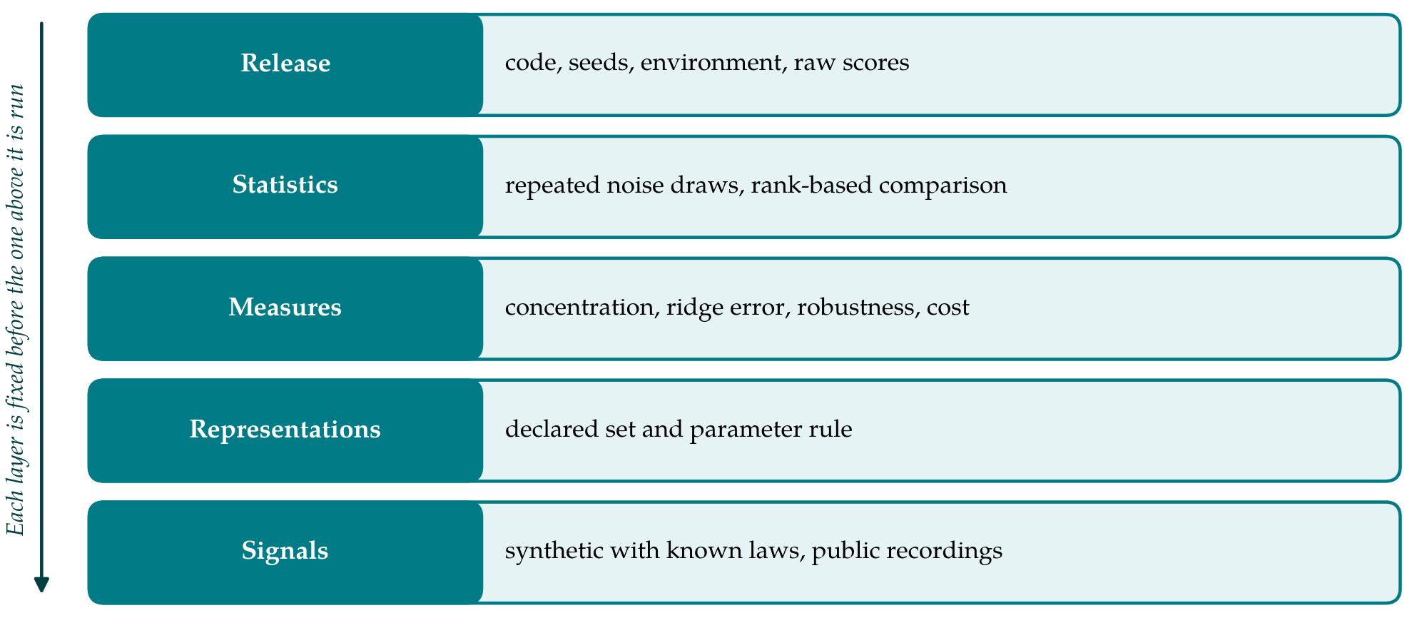
The protocol is organised as five layers, each of which is fixed before the next is run. Figure 1 shows the layers and Table 1 states what each must specify and what it must deliver.

Table 1: What each layer of the proposed protocol must specify and what it must deliver
Layer	Must be specified	Must be delivered
1. Signals	Formulas, sampling rate, duration, seeds; identifiers of recorded files	Signal generator script; ground-truth frequency laws
2. Representations	Implementations and versions; fixed or tuned parameter rule	Parameter table for every method and signal
3. Measures	Definitions, normalisation, frequency and time grids	Function that scores any time-frequency array
4. Statistics	Noise model, signal-to-noise definition and levels, repetitions	Per-run scores; rank summary across signals
5. Release	Licence, repository, software environment	Archive that regenerates every figure and table

Figure 1: The five layers of the proposed evaluation protocol, from signals at the base to public release at the top

3.1. Layer 1: Signals

The signal set has two parts. The synthetic part consists of signals generated from written formulas with known instantaneous-frequency and amplitude laws: a linear chirp, a pair of crossing chirps, components with sinusoidal frequency modulation of several depths, a set of harmonics following a prescribed speed profile as in a run-up, and a train of decaying resonances excited at a known repetition rate to imitate a localised bearing fault. Ground truth is available by construction. The recorded part uses openly available data sets with documented test conditions. For bearings, the benchmark study of Smith and Randall (2015) on the Case Western Reserve University data is a suitable reference because it records which files are and are not diagnosable by established methods. Every signal is identified by a formula and seed or by a persistent file identifier.

3.2. Layer 2: Representations and parameters

The list of representations under comparison is declared in advance, with a named implementation and version for each. The harder requirement concerns parameters. Window length, wavelet centre frequency, smoothing kernels and sifting stop criteria change the result as much as the choice of method does. The protocol asks for a written parameter rule applied identically to every method. Two rules are acceptable. Under a fixed rule, each method uses one setting chosen from its original publication for all signals. Under a tuned rule, each method is tuned by the same search procedure on a tuning subset of signals that is then excluded from scoring. Hand tuning on the scored signals is not permitted, and the search grid is published. Whichever rule is adopted, the proposed method and its competitors are bound by it equally, and the paper states which rule was used.

3.3. Layer 3: Measures

Four measures are proposed. Concentration is scored without reference to ground truth by the Rényi entropy of the normalised representation (Baraniuk et al., 2001) and by the norm-ratio measure of Stanković (2001); lower entropy indicates a more compact image. Because a representation can be compact and wrong, the second measure is ridge accuracy: the instantaneous frequency of each component is extracted with one declared ridge-tracking routine and compared with the known law, and the error is reported as a root-mean-square deviation in hertz or in orders. The third is robustness, the first two measures recomputed as noise is added. The fourth is computational cost, recorded as elapsed time on stated hardware together with the asymptotic complexity. For invertible representations a reconstruction error after mode extraction may be added. All measures are computed on common time and frequency grids, since entropy values depend on the sampling of the plane.

3.4. Layer 4: Statistics

A single noisy realisation proves little. Each synthetic signal is evaluated at several signal-to-noise ratios, defined explicitly as the ratio of signal power to noise power over the whole record, and at each level the noise is redrawn many times with recorded seeds. Scores are reported as medians with interquartile ranges, not as single values. To compare methods across the whole signal set, the rank-based procedure recommended by Demšar (2006) for comparing classifiers over multiple data sets transfers directly: methods are ranked on each signal, average ranks are tested for overall difference, and pairwise differences are examined only if the overall test rejects equality. This guards against declaring a winner on the strength of one favourable signal.

3.5. Layer 5: Release

The final layer is the publication of everything needed to regenerate the results: the signal generator, wrappers for each representation, the scoring functions, the seeds, the raw per-run scores and a description of the software environment with library versions. A single entry script should rebuild every table and figure. The archive is deposited in a repository that issues a persistent identifier and is released under an open licence. A new method can then be added to the comparison by anyone, under the same rules, without rerunning or reinterpreting the earlier ones. Random number generators deserve particular care, because their streams can differ between library versions; storing the generated noise records, or at least checksums of them, removes that source of disagreement.

4. Fitting the Protocol to Practice

The full protocol is more work than a row of spectrograms, and a proportionate version is useful. A minimum form keeps the synthetic signals, the fixed parameter rule, the two concentration measures and ridge accuracy at a few noise levels, and it still requires release. Recorded data and tuned parameters can be added when a paper's claims depend on them. Laboratories that hold proprietary recordings can follow the protocol on the public part and report the private results separately, labelled as not reproducible by readers. Journals and reviewers can use Table 1 as a checklist.

Order tracking deserves a remark, because much rotating-machinery analysis is done after resampling the signal to the shaft angle. A representation computed in the order domain faces an easier problem, since speed-related components become stationary. Where a paper compares methods on run-up or coast-down signals, it should state whether a tachometer reference was used and apply the same pre-processing to every method, so that differences in the results reflect the representations and not the preparation of their inputs.

5. Limitations and What Remains to Be Shown

The protocol is proposed here and has not been exercised on any set of methods, so its practical burden and its power to discriminate among methods are unknown. A first application would show whether the measures agree with one another and with expert judgement of the images, and whether rankings are stable under reasonable changes to the signal set. It would also show how many noise realisations are needed before the medians settle, a number that determines the computing time and that this article does not attempt to fix in advance.

Several limitations can be anticipated. Synthetic signals with clean frequency laws favour methods built on the same signal model, and real vibration contains modulation, noise and transfer-path effects that formulas capture poorly. Ridge accuracy depends on the ridge tracker, and fixing one tracker for all methods is fair without being neutral. Concentration measures reward compactness whether or not the compact energy is correctly placed. Most importantly, a sharper representation is not automatically a better diagnostic. The link from representation quality to fault detection or severity estimation requires labelled data and a task-level evaluation that lies beyond this protocol.

6. Conclusion

Comparisons of time-frequency representations for vibration signals will remain anecdotal until the signals, parameter rules, measures and code behind them are shared. The five-layer protocol proposed in this article sets out one way of doing so, using synthetic signals with known ground truth, public recordings, quantitative measures, repeated trials with rank-based statistics and full release. Its adoption, in whole or in the minimum form, would let results from different groups be placed side by side, which present practice does not allow.

Conflict of interest

To be declared by the author(s) before publication.

Funding

To be declared by the author(s) before publication.

References

[1] Antoni, J. The spectral kurtosis: A useful tool for characterising non-stationary signals. Mechanical Systems and Signal Processing https://doi.org/10.1016/j.ymssp.2004.09.001 20(2), 282-307 (2006).
[2] Auger, F. and Flandrin, P. Improving the readability of time-frequency and time-scale representations by the reassignment method. IEEE Transactions on Signal Processing https://doi.org/10.1109/78.382394 43(5), 1068-1089 (1995).
[3] Auger, F., Flandrin, P., Lin, Y.-T., McLaughlin, S., Meignen, S., Oberlin, T. and Wu, H.-T. Time-frequency reassignment and synchrosqueezing: An overview. IEEE Signal Processing Magazine https://doi.org/10.1109/MSP.2013.2265316 30(6), 32-41 (2013).
[4] Baraniuk, R.G., Flandrin, P., Janssen, A.J.E.M. and Michel, O.J.J. Measuring time-frequency information content using the Rényi entropies. IEEE Transactions on Information Theory https://doi.org/10.1109/18.923723 47(4), 1391-1409 (2001).
[5] Boashash, B. Estimating and interpreting the instantaneous frequency of a signal. I. Fundamentals. Proceedings of the IEEE https://doi.org/10.1109/5.135376 80(4), 520-538 (1992).
[6] Buckheit, J.B. and Donoho, D.L. WaveLab and reproducible research. Wavelets and Statistics (Lecture Notes in Statistics, vol. 103), Springer, New York 55-81 (1995).
[7] Cohen, L. Time-frequency distributions: A review. Proceedings of the IEEE https://doi.org/10.1109/5.30749 77(7), 941-981 (1989).
[8] Daubechies, I., Lu, J. and Wu, H.-T. Synchrosqueezed wavelet transforms: An empirical mode decomposition-like tool. Applied and Computational Harmonic Analysis https://doi.org/10.1016/j.acha.2010.08.002 30(2), 243-261 (2011).
[9] Demšar, J. Statistical comparisons of classifiers over multiple data sets. Journal of Machine Learning Research 7, 1-30 (2006).
[10] Feng, Z., Liang, M. and Chu, F. Recent advances in time-frequency analysis methods for machinery fault diagnosis: A review with application examples. Mechanical Systems and Signal Processing https://doi.org/10.1016/j.ymssp.2013.01.017 38(1), 165-205 (2013).
[11] Huang, N.E., Shen, Z., Long, S.R., Wu, M.C., Shih, H.H., Zheng, Q., Yen, N.-C., Tung, C.C. and Liu, H.H. The empirical mode decomposition and the Hilbert spectrum for nonlinear and non-stationary time series analysis. Proceedings of the Royal Society of London A https://doi.org/10.1098/rspa.1998.0193 454(1971), 903-995 (1998).
[12] Peng, R.D. Reproducible research in computational science. Science https://doi.org/10.1126/science.1213847 334(6060), 1226-1227 (2011).
[13] Randall, R.B. and Antoni, J. Rolling element bearing diagnostics: A tutorial. Mechanical Systems and Signal Processing https://doi.org/10.1016/j.ymssp.2010.07.017 25(2), 485-520 (2011).
[14] Smith, W.A. and Randall, R.B. Rolling element bearing diagnostics using the Case Western Reserve University data: A benchmark study. Mechanical Systems and Signal Processing https://doi.org/10.1016/j.ymssp.2015.04.021 64-65, 100-131 (2015).
[15] Stanković, L. A measure of some time-frequency distributions concentration. Signal Processing https://doi.org/10.1016/S0165-1684(00)00236-X 81(3), 621-631 (2001).
[16] Vandewalle, P., Kovačević, J. and Vetterli, M. Reproducible research in signal processing. IEEE Signal Processing Magazine https://doi.org/10.1109/MSP.2009.932122 26(3), 37-47 (2009).
[17] Wilkinson, M.D., Dumontier, M., Aalbersberg, I.J., et al. The FAIR Guiding Principles for scientific data management and stewardship. Scientific Data https://doi.org/10.1038/sdata.2016.18 3, 160018 (2016).

Article metrics

0 total accesses since publication. 0 citing articles have been indexed to date.