1. Introduction
Roughness is the pavement condition measure that road users feel directly and that most strongly drives vehicle operating costs, which is why it sits at the centre of pavement management models (Paterson, 1987). Since the international experiment organised by the World Bank in the 1980s it has been reported almost everywhere as the International Roughness Index (IRI), a statistic computed from the longitudinal profile of a wheel path (Sayers et al., 1986a). Specifications built on the index are now in use across the world (Múčka, 2017).
Measuring the profile requires an inertial profiler or an equivalent reference device (ASTM, 2009). Agencies deploy such equipment on their primary networks on a regular cycle. Secondary roads, which are longer in total, carry less traffic and are often the responsibility of local bodies with small budgets, are surveyed rarely or by visual rating alone. Smartphones offer a way to fill the gap. They contain accelerometers, gyroscopes and satellite positioning, they are already travelling the network in large numbers, and early demonstrations showed that road anomalies can be detected from them (Eriksson et al., 2008; Mohan et al., 2008).
This article sets out a procedure for estimating segment-level roughness from smartphone recordings contributed by volunteer drivers, with secondary roads specifically in mind. It is a proposed method. No field data are reported, and the procedure has not been validated here.
2. Background
The procedure rests on the definition of the index, on what is known about vehicle response as a proxy for it, and on the lessons of earlier smartphone studies.
2.1. The index and its reference measurement
The IRI is defined by a mathematical model, not by an instrument. A measured profile is passed through a quarter-car simulation with a fixed set of parameters travelling at 80 km/h, and the accumulated suspension travel is divided by the distance covered, giving a slope in metres per kilometre (Sayers, 1995; ASTM, 2008). The quarter-car acts as a band-pass filter that responds to the wavelengths which disturb a moving vehicle (Sayers and Karamihas, 1998). The World Bank guidelines distinguish methods that measure the profile precisely from those that record the response of a vehicle and convert it to IRI by calibration (Sayers et al., 1986b). Any smartphone method belongs to the second, response-type family, and inherits its need for calibration.
2.2. Vehicle response as a proxy
The vertical acceleration of a vehicle body is the road profile filtered by tyres and suspension and scaled by speed. Road profiles are commonly described by a power spectral density that falls with spatial frequency, the description standardised for vehicle dynamics work (ISO, 2016), and under that description the acceleration response of a linear vehicle rises with speed in a predictable way. González et al. (2008) showed by simulation that profile spectra, and hence roughness class, can be recovered from body accelerations when the transfer function of the vehicle is known. In crowdsourcing it is not known, which is the central difficulty.
2.3. Earlier smartphone studies
After the first anomaly-detection systems, which targeted potholes and bumps, attention moved to continuous roughness. Douangphachanh and Oneyama (2013) related the magnitude of acceleration recorded by phones to reference roughness and found the relation to depend on speed and vehicle. Islam et al. (2014) integrated phone accelerations to an approximate profile and computed the index from it, while commercial applications have estimated roughness directly from vibration with settings for broad vehicle classes. Bridgelall (2014) proposed a speed-normalised index from inertial and position data intended for aggregation over many connected vehicles. A review by Sattar et al. (2018) concluded that phone placement, speed and vehicle type remain the main obstacles to transferable results.
3. The Proposed Procedure
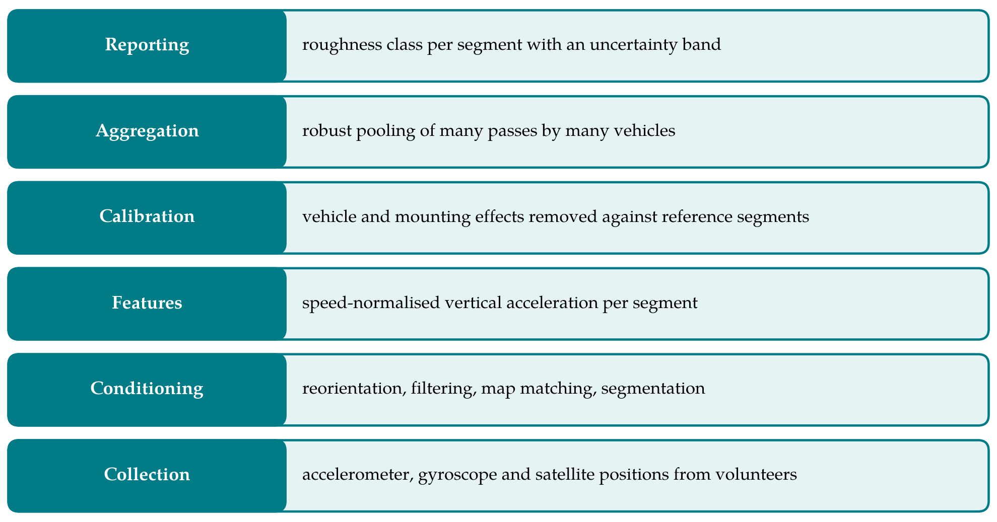
The procedure is organised as six stages, drawn as a stack in Figure 1 with collection at the base and reporting at the top. Table 1 lists the sources of unwanted variation that the stages are designed to control. The remainder of this section describes each stage.
| Source of variation | Effect on the signal | Treatment in the procedure |
|---|---|---|
| Travel speed | Acceleration rises with speed on the same road | Speed stored per pass; normalised in calibration (Stages 3-4) |
| Vehicle suspension and tyres | Different gain and resonances between vehicles | Vehicle-specific calibration on reference segments (Stage 4) |
| Phone orientation and mounting | Vertical axis misaligned; loose phones rattle | Reorientation to vehicle frame; unmounted trips flagged (Stages 1-2) |
| Position error | Features assigned to the wrong segment or road | Map matching and fixed 100 m segments (Stage 2) |
| Wheel path and lane | Vehicles sample different lines along the road | Pooling of many passes; median per segment (Stage 5) |
| Driver behaviour | Braking, swerving round defects, speed humps | Passes with unsteady speed discarded (Stage 3) |
| Handset hardware | Sampling rate and sensor noise differ | Resampling to a common rate; device recorded (Stages 1-2) |
3.1. Stage 1: Collection
Volunteers install an application that records three-axis acceleration and rotation rate at the highest stable rate the handset supports, together with satellite position, speed and heading at their native rate. Recording starts when driving is detected and stops when it ends. Each trip carries an anonymous device identifier and a persistent, anonymous identifier for the vehicle and mounting arrangement, since calibration in Stage 4 is specific to that combination. Contributors are asked to keep the phone in a fixed cradle; recordings from pockets or loose on a seat are accepted but flagged. Trip ends are trimmed before upload so that home and work locations are not disclosed.
3.2. Stage 2: Signal conditioning
The phone axes must be rotated into the vehicle frame. The direction of gravity, taken from the low-frequency part of the accelerometer signal, gives the vertical; the horizontal axes are resolved from acceleration during braking and speeding up on straight sections, a technique used since the earliest systems (Mohan et al., 2008). The vertical component is then high-pass filtered to remove gravity and slow drift. Positions are matched to the road network with a hidden Markov model map-matching algorithm, which tolerates the sparse and noisy fixes typical of handsets (Newson and Krumm, 2009), and the trace is cut into fixed segments of 100 m. Samples between position fixes are located by interpolating distance from speed.
3.3. Stage 3: Feature extraction
For each pass over each segment the procedure computes the root mean square of vertical acceleration and its power in a small number of frequency bands, the latter estimated by averaged periodograms (Welch, 1967). Bands are used because roughness, body bounce and axle hop occupy different parts of the spectrum, and a regression on several bands can discount the part dominated by the vehicle. Mean speed and its variation over the segment are stored with the features. Passes are discarded where speed is very low or changes sharply, because the response is then governed by braking and manoeuvring; the thresholds are to be fixed during validation and are deliberately not specified here.
3.4. Stage 4: Calibration
Calibration converts features to an estimate of IRI. A set of reference segments, chosen to span the range of roughness and the surface types of the secondary network, is measured with an inertial profiler and its IRI computed by the standard practice (ASTM, 2008). Contributing vehicles that traverse those segments supply paired observations. The procedure proposes a regression of the logarithm of reference IRI on the logarithms of band powers and speed, with an offset for each vehicle and mounting combination. The speed term carries the normalisation, and the offset absorbs the gain of the individual suspension. A vehicle that has never crossed a reference segment can still be calibrated indirectly, through segments it shares with vehicles that have, in the manner of the fleet aggregation envisaged by Bridgelall (2014).
3.5. Stage 5: Aggregation
A single pass is a poor estimate: the vehicle may have straddled a defect, changed line or been passing a parked car. The value assigned to a segment is therefore the median of the calibrated estimates from all accepted passes within a time window, with a minimum number of passes and of distinct vehicles before any value is published. The spread of the passes yields an interval about the median. On quiet secondary roads the window may need to be several months long to reach the minimum, and the date range should be reported with the value.
3.6. Stage 6: Reporting
Results are reported as roughness classes, for example good, fair, poor and very poor, defined by ranges of IRI appropriate to the road category, with the interval from Stage 5 determining whether a segment is assigned firmly or marked as borderline. Classes are preferred to point values because the achievable precision of a response-type estimate does not justify more, and because the purpose is to direct limited survey and maintenance resources to the right roads.
4. Considerations Specific to Secondary Roads
Secondary roads strain the assumptions of the index. Vehicles often travel well below the 80 km/h of the reference simulation, so the wavelengths that excite the vehicle differ from those that dominate the IRI; the frequency-band features of Stage 3 are intended to mitigate this, though how well they do so is an empirical matter. Surfaces are more varied, including surface dressings, patched sections and unsealed lengths, and localised defects contribute more of the roughness than on highways. Drivers who know a road steer round its worst parts. Traffic is light, so fewer passes are available, and tree cover or terrain can degrade positioning. Each of these argues for conservative reporting and for calibrating on reference segments drawn from the secondary network itself.
5. Limitations and Validation Still Required
The procedure is untested, and several of its elements may not survive contact with data. The first requirement is a validation in which estimates for segments held out of calibration are compared with profiler measurements, reporting both the error in IRI and the rate at which segments are placed in the correct class. The second is a study of how accuracy grows with the number of passes and vehicles, which determines whether the method is workable on low-volume roads at all. The third is a check of transferability: whether a calibration built in one district holds in another with a different vehicle fleet and surface mix.
Some limits are inherent. A response-type estimate cannot separate the two wheel paths, cannot recover the profile, and will not meet the precision classes defined for profilers (ASTM, 2009). Volunteers are not a random sample of traffic, and roads they avoid will stay unmeasured. The method should be regarded as a screening layer beneath conventional surveys.
6. Conclusion
Crowdsourced smartphone data can plausibly supply roughness information for roads that are otherwise seldom surveyed, provided the uncontrolled influences of vehicle, speed and handset are handled explicitly. The six-stage procedure proposed here does this through reorientation and map matching, speed-aware spectral features, calibration against a modest set of profiled reference segments, and pooling across passes, and it reports classes with uncertainty in place of single figures. Whether the resulting accuracy is sufficient for network screening is the question a field validation must now answer.
Conflict of interest
To be declared by the author(s) before publication.
Funding
To be declared by the author(s) before publication.