1. Introduction
An irrigation advisory service tells farmers when and how much to irrigate. Its conventional basis is the crop coefficient method: reference evapotranspiration is computed from weather data and multiplied by a coefficient for the crop and its growth stage (Allen et al., 1998). The method estimates what a healthy, well-watered crop would use. It cannot say what a particular field is using, and fields differ in sowing date, stand, soil and the irrigation they have already received. An adviser working from tables therefore issues the same recommendation to farmers whose crops are in quite different states.
Thermal remote sensing addresses this gap directly. Evaporation consumes energy, so a surface that is evaporating freely stays cooler than one that is not, and surface temperature observed from orbit carries information about the actual rate of evapotranspiration (ET). Models that exploit this have been in use for more than two decades (Kalma et al., 2008). What has changed is access. Landsat thermal imagery is free, global weather reanalyses are published openly, cloud platforms remove the need for local computing (Gorelick et al., 2017), and open implementations of the main models exist (Laipelt et al., 2021; Melton et al., 2022).
This article sets out a procedure for using these resources in an advisory service. It is a proposal and has not been applied or validated here; no ET maps or accuracy figures are reported. The aim is to give a service that is considering the approach a reasoned sequence of steps and a clear view of what the result can and cannot support.
2. Background
Two matters need to be understood before the procedure is described: how surface temperature is converted to ET, and what the open sensors provide. The sensors are listed in Table 1 and discussed after the models that use them.
| Source | Thermal resolution | Revisit | Role in the procedure |
|---|---|---|---|
| Landsat 8 and 9 | About 100 m, delivered at 30 m | 16 days each, 8 days combined | Primary input to the energy balance |
| ECOSTRESS | About 70 m | Irregular, varying time of day | Additional scenes between Landsat dates |
| MODIS (Terra, Aqua) | About 1 km | Daily | Temporal pattern for fusion; regional context |
| VIIRS | 375 m to 750 m | Daily | As for MODIS |
| Sentinel-3 SLSTR | About 1 km | Near daily | As for MODIS |
| Sentinel-2 | None (optical, 10 to 20 m) | About 5 days | Vegetation cover, sharpening, field checks |
2.1. Evapotranspiration from the surface energy balance
The energy available at the land surface is the net radiation less the heat conducted into the soil. It is divided between sensible heat, which warms the air, and latent heat, which evaporates water. Latent heat flux is therefore obtained as a residual: net radiation minus soil heat flux minus sensible heat flux. Net radiation and soil heat flux can be estimated from optical and thermal imagery with fair confidence. The difficulty is sensible heat, which depends on the small difference between surface and air temperature and on aerodynamic resistance.
The models differ mainly in how they handle that difficulty. SEBAL calibrates the temperature difference within each scene from two anchor pixels, one wet and cool where sensible heat is taken as negligible and one dry and hot where latent heat is taken as zero (Bastiaanssen et al., 1998). METRIC keeps this internal calibration and ties the cold anchor to reference ET computed from weather data, expressing the result as a fraction of reference ET (Allen et al., 2007). SSEBop simplifies further by predefining the cold and hot limits for each pixel, which removes the need to choose anchors and suits routine operation (Senay et al., 2013). Two-source models treat soil and canopy separately and are physically more complete but require more inputs (Norman et al., 1995).
2.2. Open data sources
Among the open sensors relevant to the task (Table 1), no single one combines fine resolution with frequent revisit. The thermal instruments on Landsat 8 and 9 observe at about 100 m and are distributed resampled to the 30 m grid of the optical bands; each satellite returns every 16 days, and the pair together every 8. ECOSTRESS, mounted on the International Space Station, observes at comparable resolution at varying times of day (Fisher et al., 2020). Daily thermal sensors resolve about a kilometre, far coarser than most irrigated fields. Sentinel-2 carries no thermal band but supplies frequent optical imagery at 10 to 20 m, useful for vegetation cover and for sharpening.
3. The Proposed Procedure
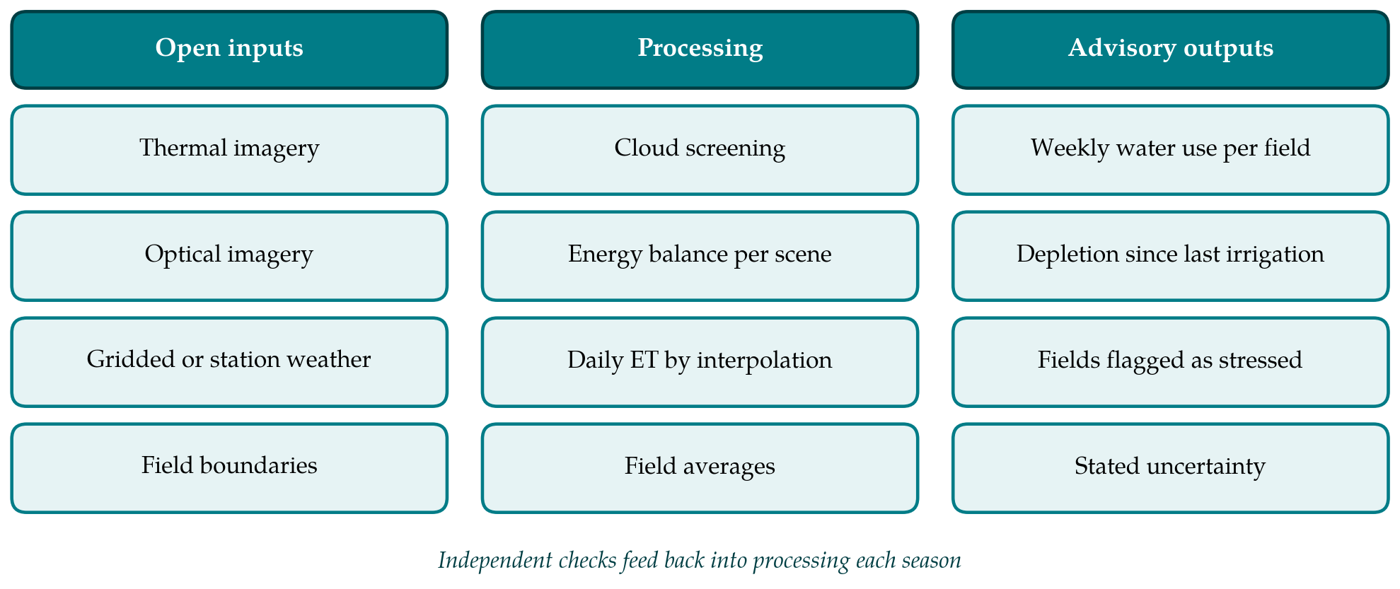
The procedure has seven steps. Figure 1 groups them by the inputs they draw on, the processing they involve and the outputs that reach the adviser. The description assumes a service covering an irrigation district or a group of villages, staffed by one or two people with training in geographic information systems.
3.1. Step 1: Define the fields and the advisory question
The service should begin with what it intends to tell farmers. A weekly statement of crop water use per field, to be set against irrigation applied, is the least demanding product. Identifying fields that are under stress is more demanding, and real-time scheduling is beyond what cloud-prone imagery at 8-day intervals can support. Field boundaries are needed to turn pixels into advice. They can be digitised from high-resolution imagery or taken from cadastral records. Fields narrower than the native thermal pixel should be marked, because their estimates will be mixed with those of their neighbours.
3.2. Step 2: Assemble imagery and weather data
Landsat surface temperature and surface reflectance products form the core. Weather data are needed for reference ET and for the energy balance itself: air temperature, humidity, wind speed and solar radiation. Where a quality-controlled station lies within the district it should be used. Where there is none, a global reanalysis such as ERA5 supplies the variables on a grid (Hersbach et al., 2020), with the caveat that reanalysis describes regional conditions and may not capture the cooler, more humid air over an irrigated area.
3.3. Step 3: Screen clouds and prepare surface temperature
Clouds and their shadows corrupt surface temperature, and thin cirrus that barely shows in the optical bands can lower it appreciably. The quality bands delivered with Landsat products, derived from the Fmask algorithm (Zhu and Woodcock, 2012), should be applied with a buffer around detected clouds. Scenes in which the district is mostly obscured are discarded. Where fields are small, the thermal band may be sharpened using its relationship with vegetation indices at finer resolution (Kustas et al., 2003; Gao et al., 2012). Sharpening redistributes temperature within a coarse pixel and does not add independent information, and it performs poorly where irrigation and vegetation cover are not well correlated, as over freshly wetted bare soil.
3.4. Step 4: Solve the energy balance for each clear scene
The choice of model should follow the capacity of the service. A model with internal calibration is tolerant of bias in the temperature product but depends on the selection of anchor pixels, which in early implementations required an experienced analyst and is now commonly automated by statistical rules. A model with predefined limits needs no such selection and is easier to run unattended, at some cost where its assumptions about the hot and cold limits do not hold. For a first season the article recommends running one automated open implementation without modification and recording the software version and settings for every scene, so that results can be reproduced. The output of this step is the ratio of actual to reference ET at the time of overpass.
3.5. Step 5: Extend from the overpass to days and weeks
A satellite observes an instant. Daily ET is obtained by assuming that the ratio of actual to reference ET at overpass holds for the whole day and multiplying by daily reference ET (Allen et al., 2007). Between clear scenes the ratio is interpolated in time for each pixel and multiplied by reference ET for each day. Interpolation is the weakest link of the chain. It cannot see an irrigation, a rain or a harvest that falls between two images, and in a cloudy season the gaps may last several weeks. Fusion with daily coarse-resolution imagery, in which the fine spatial pattern of Landsat is combined with the temporal pattern of a kilometre-scale sensor, can narrow the gaps (Gao et al., 2006; Cammalleri et al., 2013), although it adds considerable complexity and is better left to a second phase.
3.6. Step 6: Aggregate to fields and convert to advice
Pixel values are averaged within each field boundary after removing pixels that straddle the edge. The weekly total is then set beside rainfall and, where known, the irrigation applied, to give a running estimate of root-zone depletion in the manner of the standard soil water balance (Allen et al., 1998). The message to the farmer should be expressed in the units the farmer works in, such as hours of pumping or number of canal turns, and should state how many days old the latest clear image is.
3.7. Step 7: Check against independent data
No ET map should be used for advice without some independent check in the district concerned. Eddy covariance towers are the reference but are rare, and they carry uncertainty of their own because the measured fluxes commonly fail to close the energy balance (Foken, 2008; Twine et al., 2000). More accessible checks include a soil water balance on a few instrumented fields, comparison of seasonal totals with measured canal or pump deliveries, and the simple test that well-watered full-cover crops return values near reference ET. Disagreement should lead back to Step 4.
4. Fitting the Procedure to an Advisory Service
Three practical points bear on adoption. The work is seasonal and repetitive, so scripts should be written once and run unchanged, with a short log kept for each scene. Timeliness matters more than refinement: a map delivered within a few days of the overpass is of more use to an adviser than a better one delivered after a fortnight. Communication of uncertainty is part of the product. Farmers and canal managers will weigh the advice against their own observation, and an estimate presented with its age and a plain statement of confidence is more likely to keep their trust than one presented as a measurement.
5. Limitations and What Remains to Be Shown
The procedure is assembled from published methods and has not been tested as a whole. Its performance in a given district would need to be established on at least three counts: agreement of field-scale weekly ET with independent estimates over a full season; the fraction of weeks in which a usable image is available during the main irrigation period; and whether advice based on the maps changes irrigation practice. The published accuracy of thermal ET models comes largely from sites with good weather data and large uniform fields (Kalma et al., 2008), and it should not be assumed for smallholder landscapes.
Some limits are structural. Thermal sensors do not see through cloud, which rules out the method for much of a monsoon season. The native resolution of open thermal data exceeds the width of many smallholder plots. The models estimate what has been evaporated and not what should be applied, so conveyance and application losses must be added separately. Continuity of the satellite missions on which the service depends is outside its control.
6. Conclusion
Open thermal imagery, open weather data and open software have brought field-scale ET mapping within the reach of advisory services that could never have afforded it. The procedure proposed here orders the work into seven steps, recommends starting with an unmodified automated model and a modest advisory product, and treats independent checking and the honest reporting of image age and uncertainty as part of the method. Its usefulness for irrigation advice in a particular setting remains to be demonstrated there.
Conflict of interest
To be declared by the author(s) before publication.
Funding
To be declared by the author(s) before publication.