International Journal of Neural Networks and Artificial Intelligence

A Reproducible Benchmark Protocol for Evaluating Calibration in Medical Image Classifiers

Sona Khachatryan¹, Chloe Mthembu², Shanice Grigoryan³

¹ Department of Electrical Electronics, Bharathapuzha Center for Electrical Electronics, Bahrain, ² Department of Electrical Electronics, Yangtze University Centre for Electrical Electronics, Denmark, ³ Department of Electrical Electronics, Balkan Academy of Electrical Electronics, Nepal

Published 07 Jul 2026 Vol. 1, Article 3 10.62715/ijnnai.2026.v1.i1.pp15-20 0 accesses 0 citations

Download PDF XML HTML EPUB

0Accesses

0Citations

Abstract

A classifier that reports a probability of disease is useful to a clinician only if that probability can be taken at face value. Many remedies for the overconfidence of deep networks have been published, yet calibration results for medical image classifiers are difficult to compare across papers. Studies differ in how the data were split, which metric was computed, how many bins it used, whether the recalibration step saw the test data, and whether any interval accompanies the reported value. This article proposes a benchmark protocol intended to remove those sources of disagreement. It has seven steps: declare the task and fix patient-level splits, including a split reserved for recalibration; train under a stated recipe with several random seeds; fit post-hoc calibrators only on the reserved split; compute a small core set of metrics that includes proper scoring rules; attach bootstrap intervals resampled by patient; repeat the evaluation under distribution shift and within subgroups; and release the code, splits and predictions. Each step is given with its rationale and the record it should leave. The protocol is a proposal drawn from the statistical and machine learning literature. It has not been applied or validated here, and the article states what would have to be shown before it could serve as a standard.

Keywords: Calibration Reproducibility Medical image classification Expected calibration error Proper scoring rules Benchmark protocol

1. Introduction

A model that assigns a probability of 0.8 to malignancy is calibrated if, among all the images to which it assigns 0.8, about four in five are malignant. Discrimination, the ability to rank diseased cases above healthy ones, is a different property, and a model can have one without the other. For decisions that depend on thresholds, such as whether to refer, to biopsy or to reassure, the probability itself is the input, and a miscalibrated probability can mislead even when ranking is excellent. Van Calster et al. (2019) called calibration the Achilles heel of predictive analytics for this reason, and the TRIPOD reporting guideline asks that it be reported for every clinical prediction model (Collins et al., 2015).

Deep image classifiers present a particular difficulty. Guo et al. (2017) showed that modern networks tend to be overconfident and that a one-parameter rescaling of the logits, temperature scaling, corrects much of the error on data like the training set. Many alternatives followed. What has not followed is a common way of testing them in medical imaging. Two papers that both report an expected calibration error for a chest radiograph classifier may have used different bins, different splits and different rules about what the recalibration step was allowed to see.

This article proposes a protocol for benchmarking calibration in medical image classifiers so that results from different groups can be set side by side. The protocol is assembled from established statistical practice and published machine learning methods. It is offered as a proposal and has not been applied to any dataset in this article; no results are reported.

2. Background

The design rests on three bodies of prior work: how calibration is measured, how it is repaired, and why medical imaging strains both.

2.1. Measuring calibration

The oldest measure is the Brier score, the mean squared difference between forecast probability and outcome (Brier, 1950). Murphy (1973) showed that it separates into a reliability term, which is the calibration component, a resolution term and an uncertainty term fixed by the data. The Brier score and the negative log-likelihood are proper scoring rules: their expected value is optimised only by reporting the true probabilities (Gneiting and Raftery, 2007). They cannot be gamed, but they mix calibration with discrimination in a single figure.

The expected calibration error isolates calibration. Predictions are sorted into bins by confidence and the gap between mean confidence and observed accuracy is averaged across bins, weighted by bin size (Naeini et al., 2015). The measure is intuitive and pairs naturally with a reliability diagram. It is also fragile. Its value depends on the number of bins and on whether they have equal width or equal mass; in multi-class problems it usually examines only the top predicted class; and Nixon et al. (2019) documented how these choices alter the ranking of methods. Kumar et al. (2019) proved that the binned estimate can understate the true error of a continuous recalibration method and proposed a debiased estimator.

2.2. Repairing calibration

Post-hoc methods adjust the outputs of a trained model using held-out data. Platt scaling fits a logistic function to the scores (Platt, 1999); isotonic regression fits a monotone step function (Zadrozny and Elkan, 2002); and the two were compared across classical learners by Niculescu-Mizil and Caruana (2005). Temperature scaling is the single-parameter relative of Platt scaling for multi-class networks (Guo et al., 2017). Other methods act during training: label smoothing softens the targets (Müller et al., 2019), and averaging several independently trained networks, a deep ensemble, improves both accuracy and uncertainty estimates (Lakshminarayanan et al., 2017).

2.3. Why medical imaging strains both

Three features of clinical image data matter. Datasets are small and classes are unbalanced, so bins at high confidence for a rare disease may hold very few positive cases and any binned estimate is noisy. One patient often contributes several images, and if images from the same patient fall on both sides of a split the test is contaminated. And the deployment population differs from the development population in scanner, protocol and disease prevalence. Ovadia et al. (2019) found that calibration deteriorates as data move away from the training distribution and that post-hoc scaling tuned on in-distribution data is among the methods that degrade, a finding with obvious weight for a model carried from one hospital to another.

3. The Proposed Protocol

The protocol consists of seven steps. Table 1 lists what is fixed at each step and the record that should be published with the results, and Figure 1 shows the order in which the steps run. The steps are then described one at a time.

Table 1: Steps of the proposed benchmark protocol, the choices each fixes and the record to publish
Step	What is fixed in advance	Record to publish
1. Task and splits	Label definition; patient-level train, validation, calibration and test splits	Split files with patient identifiers hashed
2. Training	Architecture, preprocessing, augmentation, stopping rule, number of seeds	Configuration files and seeds
3. Recalibration	Methods compared; fitted on the calibration split only	Fitted parameters per model and seed
4. Metrics	Proper scores, binned and class-wise error, binning scheme	Metric code and reliability diagrams
5. Uncertainty	Bootstrap by patient; spread across seeds	Intervals for every reported value
6. Shift and subgroups	External test set; subgroups named before analysis	Results per site and subgroup
7. Release	Licence and location of artefacts	Code, splits, per-image predictions

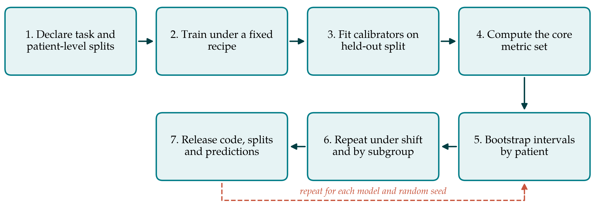
Figure 1: Order of the seven steps in the proposed benchmark protocol

3.1. Step 1: Declare the task and fix the splits

The benchmark begins with a written definition of the prediction target, including how labels were obtained and whether the problem is binary, multi-class or multi-label. Data are then divided at the level of the patient into four parts: training, validation for model selection, a calibration split used only to fit post-hoc methods, and a test split that nothing is fitted on. The fourth split is the one most often missing in published work. When recalibration parameters are tuned on the validation data that also chose the model, or on the test set itself, the reported calibration is optimistic. Split files are published so that others evaluate on identical cases.

3.2. Step 2: Train under a declared recipe

Each model is trained with a fixed and published configuration, and training is repeated with several random seeds. Calibration is sensitive to choices that are rarely reported, among them the stopping criterion, weight decay and augmentation, so these belong in the record. Repetition matters because the difference between two calibration methods can be smaller than the variation between two runs of the same method.

3.3. Step 3: Recalibrate on the reserved split

Post-hoc calibrators are fitted on the calibration split and frozen. The protocol asks for at least the uncalibrated model, temperature scaling and one non-parametric method such as isotonic regression, so that every benchmark shares a common set of reference points. Training-time methods and ensembles are entered as separate models and pass through the same later steps.

3.4. Step 4: Compute a core set of metrics

No single number is adequate, so the protocol fixes a small set. The Brier score and negative log-likelihood are reported as proper scores. Expected calibration error is reported with equal-mass bins, with the number of bins stated, together with a class-wise variant of the kind described by Nixon et al. (2019), because top-label error hides miscalibration in rare classes. A reliability diagram accompanies each model. Discrimination is reported alongside, following the framework of Steyerberg et al. (2010), who treat overall performance, discrimination and calibration as separate questions. Where the intended clinical decision is known, net benefit from decision curve analysis may be added (Vickers and Elkin, 2006).

3.5. Step 5: Quantify uncertainty

Every reported value carries an interval. The protocol specifies a nonparametric bootstrap of the test set (Efron and Tibshirani, 1993) in which patients, not images, are resampled, so that correlated images from one person stay together. Variation across training seeds is reported separately, since it answers a different question: the bootstrap describes uncertainty about this model's calibration, and the seeds describe how much the training procedure itself varies.

3.6. Step 6: Evaluate under shift and within subgroups

The metric set is computed again on at least one test set drawn from a different institution or acquisition device, without refitting the calibrators. Results are also broken down by subgroups that were named before the analysis, typically sex, age band and scanner type where the data allow. A model that is calibrated on average may be overconfident for one group and underconfident for another, and the averages conceal it. Small subgroups will have wide intervals, and the protocol asks that these be shown and not suppressed.

3.7. Step 7: Release the artefacts

The benchmark is reproducible only if its parts are available. Code for training and for the metrics, the split files, fitted calibration parameters and the per-image predicted probabilities for every model and seed are released under a stated licence. Per-image predictions are the most valuable of these, because they allow a later reader to compute a metric that the original authors did not.

4. Fitting the Protocol to Practice

The protocol adds cost in two places. Reserving a calibration split takes cases away from training, which hurts when data are scarce; cross-fitting, in which calibrators are fitted on folds held out in turn, is an acceptable substitute provided the test split remains untouched. Training with several seeds multiplies computation, and for large models a smaller number of seeds with the count stated plainly is better than a single unqualified run.

Some data cannot be shared. Where patient images are restricted, the protocol can still be followed in part by releasing code, hashed split identifiers and predictions, none of which contain images. Multi-label tasks, common in chest radiography, are handled by treating each finding as its own binary problem and reporting the metric set per finding before any average.

5. Limitations and What Remains to Be Shown

The protocol has not been tested. It is not yet known whether following it narrows the disagreement between independent groups evaluating the same method, which is its whole purpose, and that would need to be demonstrated by having several teams apply it to a shared dataset. Nor is it established that the chosen metric set is the smallest that suffices, or that equal-mass binning is the best default across the range of prevalence found in practice.

There are limits of principle as well. Calibration is assessed against labels, and in medical imaging labels carry their own uncertainty from disagreement between readers; a model may look miscalibrated against one reader and not against a consensus. The calibration measured here is what Van Calster et al. (2019) describe as moderate calibration at best, agreement on average among cases given the same predicted risk, and it says nothing certain about any individual patient. A good benchmark result is evidence about a model on particular datasets. It does not establish that the model is safe to use in a clinic, which requires prospective evaluation in the setting concerned.

6. Conclusion

Calibration results for medical image classifiers will remain hard to compare for as long as each study chooses its own splits, bins and rules of access. The seven-step protocol proposed in this article fixes those choices in advance, reserves data for recalibration, reports proper scores with patient-level intervals, looks beyond the development distribution, and makes the predictions public. Whether it delivers the comparability it aims for is an open empirical matter, and the article invites its testing.

Conflict of interest

To be declared by the author(s) before publication.

Funding

To be declared by the author(s) before publication.

References

[1] Brier, G.W. Verification of forecasts expressed in terms of probability. Monthly Weather Review 78(1), 1-3 (1950).
[2] Collins, G.S., Reitsma, J.B., Altman, D.G. and Moons, K.G.M. Transparent reporting of a multivariable prediction model for individual prognosis or diagnosis (TRIPOD): The TRIPOD statement. Annals of Internal Medicine https://doi.org/10.7326/M14-0697 162(1), 55-63 (2015).
[3] Efron, B. and Tibshirani, R.J. An Introduction to the Bootstrap. Chapman & Hall, New York (1993).
[4] Gneiting, T. and Raftery, A.E. Strictly proper scoring rules, prediction, and estimation. Journal of the American Statistical Association https://doi.org/10.1198/016214506000001437 102(477), 359-378 (2007).
[5] Guo, C., Pleiss, G., Sun, Y. and Weinberger, K.Q. On calibration of modern neural networks. Proceedings of the 34th International Conference on Machine Learning, PMLR 70: 1321-1330 (2017).
[6] Kumar, A., Liang, P. and Ma, T. Verified uncertainty calibration. Advances in Neural Information Processing Systems 32 (2019).
[7] Lakshminarayanan, B., Pritzel, A. and Blundell, C. Simple and scalable predictive uncertainty estimation using deep ensembles. Advances in Neural Information Processing Systems 30 (2017).
[8] Murphy, A.H. A new vector partition of the probability score. Journal of Applied Meteorology 12(4), 595-600 (1973).
[9] Müller, R., Kornblith, S. and Hinton, G. When does label smoothing help?. Advances in Neural Information Processing Systems 32 (2019).
[10] Naeini, M.P., Cooper, G.F. and Hauskrecht, M. Obtaining well calibrated probabilities using Bayesian binning. Proceedings of the Twenty-Ninth AAAI Conference on Artificial Intelligence 2901-2907 (2015).
[11] Niculescu-Mizil, A. and Caruana, R. Predicting good probabilities with supervised learning. Proceedings of the 22nd International Conference on Machine Learning https://doi.org/10.1145/1102351.1102430 625-632 (2005).
[12] Nixon, J., Dusenberry, M.W., Zhang, L., Jerfel, G. and Tran, D. Measuring calibration in deep learning. Proceedings of the IEEE/CVF Conference on Computer Vision and Pattern Recognition Workshops (2019).
[13] Ovadia, Y., Fertig, E., Ren, J., Nado, Z., Sculley, D., Nowozin, S., Dillon, J.V., Lakshminarayanan, B. and Snoek, J. Can you trust your model's uncertainty? Evaluating predictive uncertainty under dataset shift. Advances in Neural Information Processing Systems 32 (2019).
[14] Platt, J.C. Probabilistic outputs for support vector machines and comparisons to regularized likelihood methods. Advances in Large Margin Classifiers, MIT Press, Cambridge, MA 61-74 (1999).
[15] Steyerberg, E.W., Vickers, A.J., Cook, N.R., Gerds, T., Gonen, M., Obuchowski, N., Pencina, M.J. and Kattan, M.W. Assessing the performance of prediction models: A framework for traditional and novel measures. Epidemiology https://doi.org/10.1097/EDE.0b013e3181c30fb2 21(1), 128-138 (2010).
[16] Van Calster, B., McLernon, D.J., van Smeden, M., Wynants, L. and Steyerberg, E.W. Calibration: The Achilles heel of predictive analytics. BMC Medicine https://doi.org/10.1186/s12916-019-1466-7 17, 230 (2019).
[17] Vickers, A.J. and Elkin, E.B. Decision curve analysis: A novel method for evaluating prediction models. Medical Decision Making https://doi.org/10.1177/0272989X06295361 26(6), 565-574 (2006).
[18] Zadrozny, B. and Elkan, C. Transforming classifier scores into accurate multiclass probability estimates. Proceedings of the Eighth ACM SIGKDD International Conference on Knowledge Discovery and Data Mining https://doi.org/10.1145/775047.775151 694-699 (2002).

Article metrics

0 total accesses since publication. 0 citing articles have been indexed to date.