1. Introduction
Small direct-injection diesel engines are among the most numerous prime movers in the world. With one or two cylinders and a displacement of well under a litre, they power irrigation pumps, generator sets, small tractors and three-wheeled goods vehicles, and they are valued for low cost and tolerance of poor maintenance. Tightening emission rules and the arrival of alternative fuels now require these engines to be calibrated with more care than before, and calibration depends on knowing how combustion proceeds inside the cylinder.
The standard instrument for that purpose is a piezoelectric pressure transducer mounted in the cylinder head, with a charge amplifier and a crank angle encoder. The measurement chain is accurate but expensive, the transducer needs a machined access passage, and its life in service is limited. For a workshop, a small manufacturer or a teaching laboratory the cost is frequently out of proportion to the engine. A method that recovers even an approximate pressure trace from a signal that is cheap to measure would be useful in these settings.
Crankshaft speed is such a signal. This article describes a procedure for reconstructing cylinder pressure from the speed fluctuation of a small diesel engine with hardware that costs very little. The procedure is proposed, not demonstrated: no measurements are reported, and the closing sections state what must be tested before the method can be trusted.
2. Background
The idea is not new. What follows summarises the physical basis, the main lines of earlier work and the features of small diesel engines that make the problem both easier and harder than in automotive engines.
2.1. The torque balance
The crankshaft, flywheel and attached load form a rotating system whose angular acceleration, multiplied by its moment of inertia, equals the net torque acting on it. That net torque is the sum of the gas torque from cylinder pressure, the torque from the inertia of the reciprocating masses, friction and the load. Gas torque is the product of the pressure difference across the piston, the piston area, the crank radius and a geometric function of crank angle and connecting rod ratio (Heywood, 1988). Rizzoni (1989) cast this balance as a dynamic model and showed that indicated torque can be estimated from measured speed, which opened the field. The textbook treatments of Kiencke and Nielsen (2005) and Guzzella and Onder (2010) give the model in a form suited to implementation.
2.2. Earlier approaches
Three families of method have been published. The first inverts the torque balance directly: Citron et al. (1989) recovered pressure and torque waveforms for each cylinder from speed fluctuation with a lumped model of the crankshaft, and Moro et al. (2002) used frequency response functions relating harmonics of speed to harmonics of pressure. Taraza et al. (2001) showed that the lowest harmonic orders of speed carry the information needed for diagnosis of diesel engines. The second family uses observers, in which a model of the engine is driven by the error between measured and predicted speed (Shiao and Moskwa, 1995). The third trains a non-parametric model, such as a radial basis function network, on recorded pairs of speed and pressure (Johnsson, 2006). Connolly and Yagle (1994) supplied an idea used below: describe the pressure trace by a few parameters and estimate those, instead of estimating pressure at every crank angle.
2.3. What is particular to small diesel engines
A single-cylinder engine has no overlapping firing events, so the gas torque of one cylinder is observed without interference from its neighbours. The crankshaft is short and stiff, and torsional resonance, which complicates the problem in long multi-cylinder shafts (Schagerberg and McKelvey, 2003), lies well above the frequencies of interest. The speed fluctuation is large because one firing in two revolutions must carry the whole cycle. Against these advantages, the reciprocating inertia torque is comparable in size to the gas torque at high speed, the driven machine may impose an unsteady load, and the flywheel teeth on a low-cost engine are cut to loose tolerances.
3. The Proposed Procedure
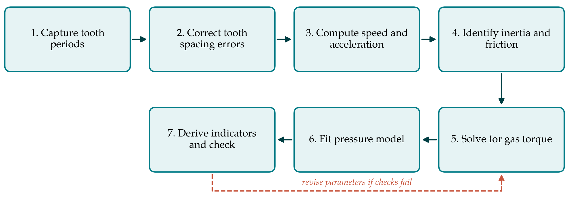
The procedure has seven steps, shown as a sequence in Figure 1. Table 1 lists what each step produces and the error source that most limits it. The hardware assumed is a Hall-effect or variable reluctance sensor facing the starter ring gear, a second sensor or a missing-tooth mark to give one reference pulse per revolution, and a microcontroller with a timer capture input.
| Step | Output | Principal error source |
|---|---|---|
| 1. Capture tooth periods | Time per tooth interval, cycle phase | Timer resolution; edge jitter |
| 2. Correct tooth spacing | Correction factor per tooth | Residual friction during coast-down |
| 3. Speed and acceleration | Smoothed acceleration against crank angle | Filter cut-off removes sharp pressure rise |
| 4. Inertia and friction | Inertia, friction and load parameters | Unsteady load; simplified friction law |
| 5. Gas torque | Gas torque and pointwise pressure | Singularity at top dead centre |
| 6. Pressure model fit | Wiebe and polytropic parameters; full trace | Model too simple for two-stage combustion |
| 7. Indicators and checks | Mean effective pressure, peak pressure and its angle | Top dead centre phasing error |
3.1. Step 1: Capture tooth periods
The microcontroller records the time between successive tooth edges with a hardware timer, so that the resolution is set by the timer clock and not by software latency. Angular resolution equals the tooth pitch, which on a typical ring gear is a few degrees of crank angle. The reference pulse identifies the tooth nearest top dead centre, and a cam or injection signal, or simply the asymmetry of the speed trace, distinguishes the compression stroke from the exhaust stroke. Records of at least a hundred consecutive cycles at steady load are stored for averaging.
3.2. Step 2: Correct tooth spacing errors
Unequal tooth spacing appears as a speed fluctuation that repeats every revolution and has nothing to do with combustion. The usual remedy, described in work on misfire detection (Kiencke, 1999), is to learn a correction factor for each tooth while the engine coasts down with fuel cut off, when the true speed changes smoothly. The factors are stored and applied to all later records. Without this step the acceleration signal is dominated by manufacturing error.
3.3. Step 3: Compute speed and acceleration
Corrected tooth periods give the mean speed over each tooth interval. Acceleration is obtained by differentiating with respect to crank angle, and differentiation amplifies noise. The record is therefore averaged over cycles first and then smoothed with a zero-phase low-pass filter whose cut-off is expressed in harmonic orders of the engine cycle. Retaining roughly the first ten to twenty orders is a reasonable starting point, since the pressure trace of a diesel engine has little energy above that range apart from the sharp rise at ignition.
3.4. Step 4: Identify inertia and friction
The moment of inertia of the rotating assembly and the reciprocating mass are taken from drawings or by weighing. Friction and load torque are harder to know. The proposal is to identify them from the compression stroke, where pressure follows a polytropic law fixed by intake conditions and compression ratio, so that the torque balance contains only the unknown resistance. A mean friction torque with a speed-dependent term, in the manner of Chen and Flynn (1965), is fitted to that interval. A more detailed description of instantaneous friction exists (Rezeka and Henein, 1984), but it has more parameters than this signal can support.
3.5. Step 5: Solve for gas torque
With inertia, reciprocating torque, friction and load accounted for, the torque balance yields the gas torque at each crank angle. Dividing by piston area, crank radius and the geometric function gives pressure. The division fails near top dead centre, where the geometric function passes through zero: the piston has no lever arm on the crank, pressure produces no torque, and any noise is amplified without limit. This is an ill-posed inverse problem in the sense treated by Hansen (1998), and it is the reason for the next step.
3.6. Step 6: Fit a low-order pressure model
Instead of accepting the pointwise result, the procedure fits a thermodynamic model with a handful of parameters to the gas torque over the whole compression and expansion interval. The model is a single-zone energy balance: polytropic compression from known intake conditions, heat release described by a Wiebe function with start, duration and shape parameters (Ghojel, 2010), and wall heat loss from a standard correlation (Woschni, 1967). The parameters are adjusted by least squares so that the gas torque predicted by the model matches the torque obtained in step 5, with the angles close to top dead centre given low weight. The fitted model then supplies the pressure where direct inversion cannot.
3.7. Step 7: Derive indicators and check consistency
From the reconstructed trace the usual indicators are computed: indicated mean effective pressure, peak pressure and its crank angle, and the angle at which half the heat has been released. Indicated mean effective pressure is sensitive to errors in the assumed position of top dead centre, as Brunt and Emtage (1996) showed for measured pressure, and the same holds here. Two checks are proposed. The indicated work should equal the measured brake work plus the friction identified in step 4, and the fitted start of combustion should fall after the known start of injection by a plausible ignition delay. If either check fails, the parameters of steps 4 and 6 are revisited.
4. Fitting the Procedure to Practice
The procedure was designed around three practical constraints. The first is cost: the sensor, the microcontroller and a serial link to a laptop are commodity parts, and no machining of the engine is required. The second is skill. Steps 1 to 3 run unattended once set up; steps 4 to 6 are a curve fit that can be scripted with open numerical libraries, and the user needs to understand the engine more than the mathematics. The third is the test condition. A steady load from a brake, a generator with a resistive bank or a pump at fixed head is assumed, because an unknown fluctuating load cannot be separated from gas torque by this method.
Some adaptations are foreseeable. Where the ring gear is inaccessible, a printed encoder strip on the flywheel rim read by an optical sensor serves the same purpose. For twin-cylinder engines with even firing intervals the same steps apply to each firing separately. For engines with pilot injection or marked premixed and diffusion phases, a double Wiebe function may be needed in step 6, at the price of more parameters and a less well-conditioned fit.
5. Limitations and What Remains to Be Shown
The procedure has not been validated here, and its limitations are structural as well as practical. Near top dead centre the speed signal contains no information about pressure, so peak pressure in particular is inferred from the model and not observed. A reconstruction can therefore look convincing while being wrong about the feature of most interest. The low-pass filtering of step 3 removes the detail of the premixed pressure rise, so the method cannot be expected to resolve combustion noise or knock-like events. Friction identified on the compression stroke is assumed to hold during expansion, when piston side thrust is higher.
A validation would compare reconstructed and measured traces on an engine fitted with a reference transducer, across speed, load and injection timing, and would report errors in indicated mean effective pressure, peak pressure and combustion phasing separately. It should establish how the errors grow with speed, where inertia torque dominates, and how sensitive the result is to the assumed top dead centre position and to the filter cut-off. It should also test whether parameters identified on one engine transfer to another of the same model. Until such results exist, the method should be regarded as a means of detecting relative changes, for example between fuels or injection settings on one engine, and not as a substitute for measurement.
6. Conclusion
The speed fluctuation of a small diesel engine carries a usable imprint of cylinder pressure, and the single-cylinder layout removes several obstacles met in automotive engines. The seven-step procedure proposed here combines tooth error correction, a torque balance and a low-order thermodynamic model so that the unobservable region near top dead centre is bridged by physical reasoning. Its hardware demands are slight. Its accuracy is an open question that only comparison with measured pressure can answer, and the design of that comparison has been outlined so that others may carry it out.
Conflict of interest
To be declared by the author(s) before publication.
Funding
To be declared by the author(s) before publication.