1. Introduction
A sample of infested wheat or rice may contain half a dozen beetle species within a few millimetres of one another in size. The commonest are the weevils of the genus Sitophilus, the lesser grain borer Rhyzopertha dominica, the flour beetles Tribolium castaneum and T. confusum, the saw-toothed grain beetle Oryzaephilus surinamensis and the flat grain beetles of the genus Cryptolestes (Rees, 2004). They differ in whether they attack sound kernels, in their tolerance of phosphine and in their regulatory status, so that management depends on knowing which are present (Hagstrum and Subramanyam, 2006). Identification is done under a stereo microscope by trained staff, of whom there are few.
Image classification by deep learning offers a way of extending that expertise. Convolutional networks learn discriminating features directly from labelled images (LeCun et al., 2015), and in entomology they have reached the accuracy of specialists on some difficult tasks (Valan et al., 2019). Reviews have set out the general promise for insect monitoring (Høye et al., 2021), and detection networks have been applied to images of insects in grain (Shen et al., 2018).
Published accuracies are, however, hard to compare and often optimistic, because they depend on how the images were collected and divided. This article proposes a procedure for developing and testing a classifier of stored-grain beetles that guards against the commoner sources of over-statement. It is a design drawn from the literature. No classifier was trained for this article, and the procedure is offered for others to apply and test.
2. Background
Two bodies of knowledge inform the design: the taxonomy of the beetles, which fixes what an image can and cannot show, and the practice of transfer learning, which fixes how much data is needed.
2.1. What can be seen in an image
Some stored-grain beetles are distinctive at a glance. Others form pairs that are separated on fine characters. Tribolium castaneum and T. confusum differ in the form of the antennal club and in the distance between the eyes on the underside of the head. Sitophilus oryzae and S. zeamais overlap in external appearance and are reliably separated only by the genitalia, and the same is true of several Cryptolestes species (Rees, 2004). The khapra beetle, Trogoderma granarium, a quarantine pest in many countries, belongs to a genus whose species are difficult even for specialists. A classifier fed dorsal photographs cannot be expected to resolve what a taxonomist resolves by dissection, and the class list has to respect that limit.
2.2. Transfer learning
The networks that transformed image recognition were trained on ImageNet, a collection of more than a million labelled photographs (Deng et al., 2009). No grain laboratory will assemble a set of that size. It does not need to, because the early layers of a network trained on general images encode edges, textures and shapes that transfer to other tasks (Yosinski et al., 2014). Fine-tuning a pretrained network on a few hundred images per class is now the standard route for species identification (Wäldchen and Mäder, 2018). Residual networks (He et al., 2016) are the usual baseline. Compact architectures such as MobileNetV2 (Sandler et al., 2018) and the EfficientNet family (Tan and Le, 2019) are attractive where the model must run on a phone or an embedded board.
3. The Proposed Procedure
The procedure has eight steps, shown in sequence in Figure 1. Table 1 sets out for each step the decision it requires and the record it should leave, so that a reader of the eventual report can judge the result.
| Step | Decision to be made | Record to keep |
|---|---|---|
| 1. Taxa and use case | Which classes; which species pairs to merge | Class list with reasons |
| 2. Specimens | Sources per class; who identifies and how | Specimen register and vouchers |
| 3. Imaging | Device, views, backgrounds and lighting | Written imaging protocol |
| 4. Data split | Which sources are held out for testing | Partition list by specimen |
| 5. Training | Architectures, augmentation, class weighting | Code, settings and random seeds |
| 6. Evaluation | Metrics; which errors matter most | Confusion matrix and per-class recall |
| 7. Calibration | Confidence below which no answer is given | Threshold and share of images declined |
| 8. Deployment | How samples are re-checked by a person | Audit log and retraining dates |
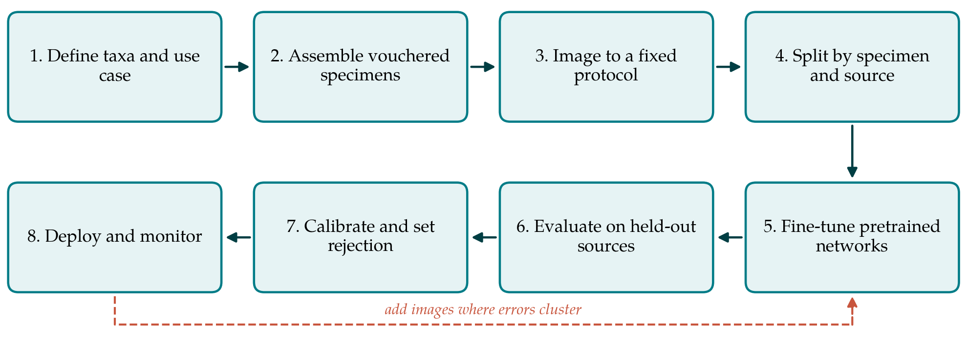
3.1. Step 1: Define the taxa and the use case
The first decision is what the classifier is for. Screening intake samples for any live insect, naming the species in a trap catch, and flagging a possible quarantine pest are different tasks with different costs of error. The class list follows from the task and from what images can show. Species that cannot be separated externally are merged into a single class named for the pair or the genus. A class for other insects and debris is included from the outset, since a deployed system will meet mites, psocids, moth larvae, fragments and weed seeds.
3.2. Step 2: Assemble vouchered specimens
Labels are only as good as the identifications behind them. Each specimen should be identified by a competent person using standard keys, with dissection where the species requires it, and should carry an identifier that links it to its images. Specimens should come from several laboratory cultures and field collections for each class. Beetles from one culture share age, diet and condition, and a network can learn the culture in place of the species.
3.3. Step 3: Image to a fixed protocol
Images should be taken with the kind of device, magnification, background and lighting that will be used in service, and those conditions should be varied deliberately across all classes. If every Rhyzopertha is photographed on white card and every Oryzaephilus on grey, the background becomes the easiest feature to learn. Several views of each specimen, dorsal, lateral and ventral, add information, and the ventral view matters for the flour beetles. Dead, damaged and dusty individuals should be included because they are what real samples contain.
3.4. Step 4: Split by specimen and by source
Dividing images at random between training and test sets is the commonest cause of inflated accuracy. Several images of one beetle are nearly duplicates, and if they fall on both sides of the split the test measures memory. All images of a specimen must go to one partition. Better still, whole sources, a culture, a collection site or an imaging session, are held out, following the argument for blocked validation of structured ecological data made by Roberts et al. (2017). The test set is then set aside and consulted once.
3.5. Step 5: Fine-tune pretrained networks
Two or three pretrained architectures of different size are fine-tuned on the training partition, with a validation partition used to choose the learning rate and the stopping point. Augmentation by rotation, flipping, cropping and changes of brightness and contrast enlarges the effective sample and suits specimens that have no natural orientation (Shorten and Khoshgoftaar, 2019). Colour should be perturbed only mildly, because the reddish brown of Tribolium against the darker Sitophilus is itself diagnostic. Classes with few images are over-sampled or weighted in the loss.
3.6. Step 6: Evaluate on held-out sources
Overall accuracy conceals what matters when classes are unequal in size and in importance. The report should give the full confusion matrix, recall and precision for each class, and an average that weights classes equally (Sokolova and Lapalme, 2009). For a regulated species the figure of interest is the proportion of true specimens that the classifier misses. Saliency maps such as Grad-CAM (Selvaraju et al., 2017) should be inspected for a sample of images to confirm that the network attends to the insect and, ideally, to the parts a taxonomist would examine.
3.7. Step 7: Calibrate and set a rejection rule
Modern networks are often over-confident, and their output scores should not be read as probabilities without adjustment. Temperature scaling on the validation set is a simple correction (Guo et al., 2017). With calibrated scores a threshold is set below which the system returns no identification and refers the specimen to a person. The same mechanism gives a first defence against species outside the training set, which tend to receive lower maximum scores (Hendrycks and Gimpel, 2017), although it is far from complete. The threshold is chosen from the cost of a wrong answer against the cost of a referral, and the share of images declined is reported with the accuracy on the remainder.
3.8. Step 8: Deploy and monitor
A classifier in service meets new cameras, new grain types and new populations. A fixed fraction of its identifications, and all referrals, should be checked by a trained person, and the agreement tracked over time. Images on which it failed are added to the training pool with verified labels, and the model is retrained at stated intervals against the same held-out test set, so that successive versions can be compared.
4. Fitting the Procedure to a Grain Laboratory
The demands of the procedure are modest in equipment and heavier in discipline. A stereo microscope with a camera port, or a phone with a clip-on macro lens, is adequate for adults of the species concerned. Training can be done on a single graphics card or a rented one. The scarce input is the taxonomist's time in step 2, and it is best spent on a few hundred well-documented specimens per class from varied sources, in preference to thousands of images of beetles from one jar. Where a laboratory handles a regulated pest, any positive from the classifier should be treated as a prompt for confirmation by the national plant protection service and never as a diagnosis.
5. Limitations and What Remains to Be Shown
The procedure has not been applied to a dataset in this article, and its benefits are argued, not demonstrated. It would need to be shown that classifiers built this way lose less accuracy when moved to a new site than classifiers built on randomly split data, and that the rejection rule catches a useful share of unfamiliar species. The treatment here is confined to adult beetles presented singly. Larvae, which do much of the damage inside kernels, mixed samples that require detection before classification, and insect fragments in flour are separate problems. Nor does image classification remove the need for dissection or molecular methods where species are externally alike; it only makes clear where that need lies.
6. Conclusion
Automated identification of stored-grain beetles from images is technically within reach of an ordinary laboratory. The risk lies less in building a classifier than in believing an accuracy figure that reflects how the data were divided. The eight steps proposed here tie the class list to what the taxonomy allows, hold out whole sources for testing, report errors class by class, and give the system a way of declining to answer. Applied and reported in this form, classifiers from different laboratories could be compared, and their performance in service could be checked against what was claimed for them.
Conflict of interest
To be declared by the author(s) before publication.
Funding
To be declared by the author(s) before publication.