1. Introduction
Neutralisation is among the simplest operations in industrial wastewater treatment to describe and among the hardest to run well. Acidic or alkaline effluent is mixed with a reagent until its pH lies within the range that the discharge permit or the downstream biological plant will accept (Eckenfelder, 2000; Metcalf & Eddy, 2014). In Europe such permits are issued under the Industrial Emissions Directive (European Parliament and Council, 2010), and comparable regimes exist elsewhere. Effluent that is out of range cannot leave the site. When the unit cannot keep up, production has to slow or stop.
Specialty chemicals plants are especially exposed. They make many products in shared equipment, each with its own washings and mother liquors, and the effluent changes in flow, acidity and buffering from one campaign to the next. A neutralisation unit sized for the original product list becomes a bottleneck as the list grows. The expensive response is to add tankage. Experience recorded in the pH control literature suggests that volume is often not the limiting factor (Shinskey, 1973; McMillan, 1994).
This article proposes a structured way of debottlenecking such a unit. It does not describe a project at any particular plant and reports no measurements. The procedure is put forward for use and for testing, and has not been validated here.
2. Why Neutralisation Units Become Bottlenecks
Three features of the process explain most capacity problems: the shape of the titration curve, the dynamics of mixing and measurement, and the variability of the load.
2.1. The titration curve and rangeability
pH is a logarithmic measure, so each unit represents a tenfold change in hydrogen ion activity. For a strong acid neutralised with a strong base the titration curve is nearly vertical around neutrality: a minute excess of reagent moves the pH by several units. To bring a strongly acidic stream into a narrow band the reagent must be metered with a precision, relative to its full flow, that is orders of magnitude beyond what a single control valve can deliver. Shinskey (1973) set out this rangeability problem and the classical answers to it: neutralise in stages, with coarse adjustment first and fine adjustment later, and use valves or pumps of different sizes in sequence.
Real effluents are seldom pure strong acids. Weak acids and bases, carbonates, phosphates and amines buffer the solution and flatten the curve, which makes control easier but raises reagent demand. Models of pH dynamics built from chemical equilibria and from reaction invariants capture this behaviour (McAvoy et al., 1972; Gustafsson and Waller, 1983), and the strong acid equivalent of Wright and Kravaris (1991) offers a way of linearising it. At a multiproduct site the difficulty is that the buffering changes with the campaign, so that controller settings which suit one effluent oscillate or respond sluggishly with another.
2.2. Mixing, dead time and measurement
A pH loop can only correct what it has seen. The delay between adding reagent and observing its effect at the electrode includes the time to disperse the reagent through the vessel, transport delay to the electrode, and the response of the electrode itself. McMillan (1994) treats the ratio of this dead time to the vessel residence time as the central design quantity: a large, poorly agitated tank has plenty of volume and still controls badly. Short-circuiting from inlet to outlet and stagnant zones make matters worse and can be diagnosed by the tracer methods of residence time distribution analysis (Levenspiel, 1999). Agitator selection and the point of reagent addition govern blend time (Paul et al., 2004). Coated or aged electrodes add a slow, drifting lag that is easily mistaken for a process problem.
2.3. Reagent behaviour
Reagents differ in speed as well as in price. Sodium hydroxide and mineral acids react almost instantly. Lime slurry is cheaper per unit of alkalinity but must dissolve before it reacts, needs longer residence time, and with sulfate-bearing effluent forms calcium sulfate scale and sludge (Eckenfelder, 2000). A unit can therefore be limited not by its vessels but by reagent preparation, by the size of a dosing pump, or by solids handling downstream.
3. A Constraint-Led Procedure
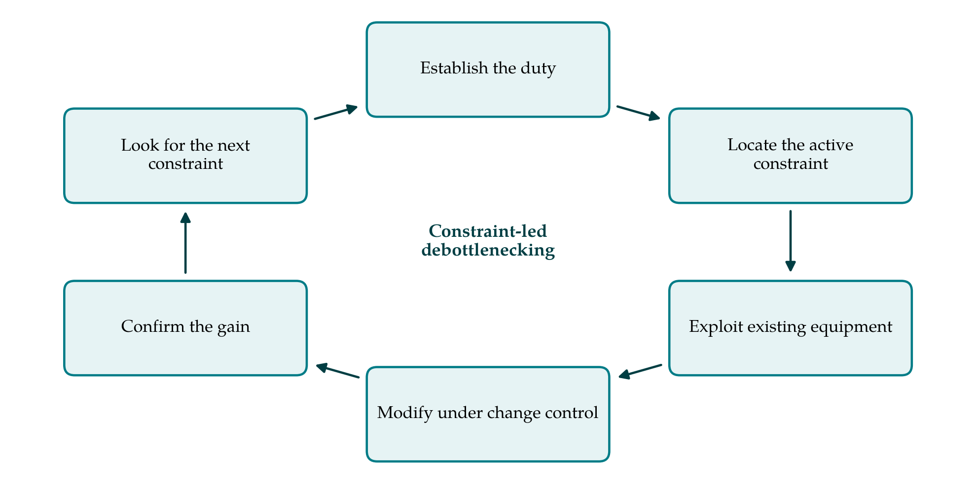
The theory of constraints holds that the output of a system is set by one limiting resource at a time, and that improvement effort spent anywhere else is wasted. Goldratt and Cox (1984) reduced this to a cycle: identify the constraint, exploit it, subordinate other decisions to it, elevate it if necessary, and then start again. The procedure proposed here applies that cycle to a neutralisation unit in five phases, shown in Figure 1. The integration of operability with design that Walsh and Perkins (1996) argued for, using effluent neutralisation as an example, is the same idea approached from the design side.
3.1. Establishing the duty
The first phase defines what the unit is being asked to do. Flow records are examined for peaks and their duration, not only for averages. Samples of the influent are taken across the campaigns that matter and titrated in the laboratory with the plant reagent, giving a family of titration curves. From these follow the range of reagent demand, the steepness of the curve at the target pH, and so the precision of reagent delivery that control within the permit band requires. The permit conditions themselves, including any averaging period, are read carefully, because a limit on an instantaneous value and a limit on a composite sample call for different designs.
3.2. Locating the active constraint
The second phase asks which element fails first as load rises. Table 1 lists the candidate constraints, the way each shows itself in operation, a diagnostic check, and the remedies that should be considered before new vessels. The checks are deliberately simple. A step test with the controller in manual gives the dead time and the process gain at the current operating point. Valve position and pump stroke records show whether reagent delivery saturates. A tracer test shows whether the working volume is the nominal volume. Comparing the on-line electrode with a freshly calibrated portable instrument separates measurement faults from process faults.
| Constraint | How it shows itself | Diagnostic check | Remedies to consider first |
|---|---|---|---|
| Mixing and dead time | Oscillation that tuning does not cure | Step test; tracer test | Relocate injection and electrode; improve agitation |
| Measurement | Slow drift; disagreement with laboratory | Check against portable meter | Cleaning routine; redundant electrodes |
| Control scheme | Good in one campaign, poor in another | Loop performance by campaign | Gain scheduling; feedforward on flow |
| Reagent kinetics and solids | pH creeps after leaving the vessel | pH of held samples over time | Longer contact time; change of reagent |
| Constraint | How it shows itself | Diagnostic check | Remedies to consider first |
|---|---|---|---|
| Hydraulic | Overflow or high level at peak flow | Flow peaks against line and pump capacity | Upstream equalisation; scheduling of discharges |
| Reagent delivery | Valve or pump at its limit; pH recovers slowly | Valve position and pump stroke records | Larger or split-range dosing; stronger reagent |
| Rangeability | Cycling between high and low pH | Titration curve slope at the target | Staged neutralisation; small trim valve |
3.3. Exploiting the existing equipment
Once the constraint is known, the third phase seeks capacity that needs no capital. Controller tuning is revisited with a method suited to processes dominated by dead time (Skogestad, 2003), and the gain is scheduled against pH or against campaign where the titration curve changes (Åström and Hägglund, 2006). Feedforward from influent flow removes the largest measurable disturbance (Seborg et al., 2016). Electrode cleaning and calibration intervals are set from observed drift. Production scheduling can be asked to avoid the simultaneous discharge of the two most demanding streams, which is subordination in Goldratt's sense: the rest of the plant adapts to the constraint while it remains one.
3.4. Modifying under management of change
If exploitation is not enough, the constraint is elevated by modification. The options, roughly in order of cost, are moving the reagent injection point or the electrode, adding a small trim valve or dosing pump, improving agitation, adding an in-line mixer with a fast loop ahead of the tank, installing upstream equalisation, and adding a further stage. More elaborate nonlinear or adaptive controllers have been demonstrated on laboratory neutralisation rigs (Henson and Seborg, 1994) and may suit a site with the skills to maintain them. Every modification, including a change of reagent, passes through the site's management of change system (CCPS, 2008) with a hazard study where warranted (IEC, 2016), since neutralisation involves corrosive reagents, heat of reaction and, with some effluents, the possibility of gas evolution.
3.5. Confirming the gain and repeating
The final phase repeats the diagnostic checks of the second under the new arrangement and at the highest load that can be arranged safely. The purpose is twofold: to confirm that the constraint addressed has moved, and to learn which element now limits the unit. A debottlenecking exercise ends when the required capacity is met with a stated margin, or when the next constraint can only be relieved by an investment that has to be justified on its own terms by the usual methods of project evaluation.
4. Where the Procedure May Not Fit
The procedure assumes that the constraint lies within the neutralisation unit. If the real limit is a permit condition on salt load, a downstream clarifier or the capacity of a municipal sewer, better pH control will not help, and the first phase should bring this to light. It also assumes that the influent can be characterised by a manageable number of titration curves. Where products change weekly and effluents are mixed unpredictably, the family of curves may be too wide for any fixed design, and segregation of streams at source becomes the more promising line.
As a proposal, the procedure carries the further limitation that its benefit has not been measured. Its value would be shown by applying it at several sites and recording, for each, which constraint was found, what was done, what the change cost, and how much capacity was gained, set against the cost of the tankage that would otherwise have been installed. Such accounts would also show whether the list of constraints in Table 1 is complete and whether the diagnostic checks discriminate between them as cleanly in practice as they do on paper.
5. Conclusion
A neutralisation unit that limits production is not necessarily too small. The chemistry of the titration curve, the dynamics of mixing and measurement, and the changing nature of specialty effluents mean that the active constraint may be reagent delivery, rangeability, dead time, instrumentation or control, each with remedies far cheaper than new vessels. The five-phase cycle proposed in this article gives a way of finding that constraint and dealing with it in order of cost. It awaits application, and reports from practitioners who try it would be the proper test of its usefulness.
Conflict of interest
To be declared by the author(s) before publication.
Funding
To be declared by the author(s) before publication.